
The Miterra Model: Integrated Modelling of Nutrient Flows at Regional or Farm Level
Yunfeng Duan 1,
Jan Peter Lesschen 1,
Chantal Hendriks 1,
Karin Nikolaus 1,
Wim de Vries 2,
Gerard Ros 2,
Mengru Wang 2,
Donghao Xu 2
1 Team Sustainable Soil Management, Wageningen Environmental Research, 6708 PB Wageningen, the Netherlands
2 Earth Systems and Global Change Group, Wageningen University, 6708 PB Wageningen, the Netherlands
Last updated: 2025-05-23 15:58:50 UTC.

|
This document is a printout of the Miterra Model Documentation webpage for offline reading and commenting. The webpage may have been updated since this printout is made. Visit https://ssm-wenr.github.io/miterra-site/ for the up-to-date content. |
- 1. Introduction
- 2. Specifications
- 3. Livestock & Manure Management
- 4. N Emissions from Manure Management
- 5. Water Fluxes
- 6. Crop Production
- 7. Fertilization
- 8. Compost & Sludge
- 9. Input To & Output From Soil
- 10. N Losses from Soil
- 11. Soil P Dynamics
- 12. Soil S Dynamics
- 13. Heavy Metal (Cd, Cu & Zn) Dynamics
- 14. Base Cation Dynamics
- 15A. The RothCN Model
- 15B. Integration of RothCN in Miterra
- 16. The ALFAM2 Model
- 17. Utility Functions
1. Introduction
Miterra is a deterministic model to simulate integrated flows and emissions of nutrient elements at various geographical scales. The model was originally developed as a regional model, named Miterra-Europe, to assess the effects and interactions of policies and measures in agriculture on N losses on a NUTS (Nomenclature of Territorial Units for Statistics) 2 level for all member states of the European Union (EU) ( Velthof et al., 2009; de Vries et al., 2011, Velthof et al., 2014). In recent projects, Miterra-Farm, a farm-level version of the Miterra model, was adapted using the same approaches of the European version, to estimate emissions and assess mitigation measures at farm scale ( Duan et al., 2023).
In general, the Miterra model can estimate:
-
Atmospheric emissions of ammonia (NH3), nitrous oxide (N2O), nitrogen oxides (NOx), and methane (CH4) from manure management and fertilization;
-
Surface runoff and leaching of N & P to the ground- and surface waters;
-
Turnover and sequestration of soil organic C and N;
-
Balance of other nutrient elements: S, K, Na, Ca & Mg; and
-
Balance of soil heavy metals (Cd, Cu & Zn).
Miterra can also model a suite of mitigation measures, and can be used to assess the effects of different management strategies and policies at farm, national, or European level.
The Miterra model comprises a comprehensive, collated input database on European climate and soil data, livestock numbers, land use, crop areas and yields, nutrient inputs and outputs, and emission factors for greenhouse gas emissions, and runoff and leaching factors for N. The model calculations are primarily based on emission factors, but also include processed-based algorithms from other models such as INTEGRATOR, RothC, and ALFAM2.
Model structure
The Miterra model can be roughly divided into 2 main components ( Figure 1.1): one capturing the flows in and emissions from the livestock sector, and the other representing the processes in the soil and the cropping sector.
In the livestock sector, N content in livestock excretions in both solid and liquid forms during housing, farmyard, storage, and grazing periods are calculated. Gaseous N emissions, including NH3, N2O, and NOx, as well as N losses to water during storage, are estimated using emission factors. Ex-storage manure and excretions during grazing are distributed to the soil as organic fertilisers.
Other nutrient inputs to soil include minerla fertilisers, crop residues, atmospheric depositions, and biological N fixation. In the soil, the uptake of nutrient elements by crop, emissions to the atmosphere, runoff and leaching to surface water and groundwater, and the turnover of soil organic matters are calculated by the model to produce a detailed budget of nutrient input, output, and balance.

Miterra was originally developed to focus on the flows of C, N, and P. Recent development has included processes to model other elements, such as S, K, Na, Ca, and Mg, as well as heavy metals Cd, Cu, and Zn. The flows of most elements are modelled independent of each other, except for the turnover of organic C and N, which are coupled via C:N ratios.
2. Specifications
Model input
| Parameter | Datasets | Sources |
|---|---|---|
Soil Properties |
||
Soil pH, CEC, availability of CaCO3, NPK content |
Soil Chemical properties at European scale based on LUCAS 2009/2012 topsoil data |
Ballabio, C., Lugato, E., Fernández-Ugalde, O., Orgiazzi, A., Jones, A., Borrelli, P., Montanarella, L. and Panagos, P., 2019. Mapping LUCAS topsoil chemical properties at European scale using Gaussian process regression. Geoderma, 355: 113912. |
Soil organic carbon (SOC) content |
LUCAS 2018 TOPSOIL data |
Fernandez-Ugalde, O; Scarpa, S; Orgiazzi, A.; Panagos, P.; Van Liedekerke, M; Marechal A. & Jones, A. LUCAS 2018 Soil Module. Presentation of dataset and results, EUR 31144 EN, Publications Office of the European Union, Luxembourg. 2022, ISBN 978-92-76-54832-4, doi:10.2760/215013, JRC129926. Orgiazzi, A., Ballabio, C., Panagos, P., Jones, A., Fernández-Ugalde, O. 2018. LUCAS Soil, the largest expandable soil dataset for Europe: A review. European Journal of Soil Science, 69(1): 140–153. https://doi.org/10.1111/ejss.12499. |
Soil texture, coarse fractions, bulk density, rooting depth |
Topsoil physical properties for Europe (based on LUCAS topsoil data) |
Ballabio C., Panagos P., Montanarella L. Mapping topsoil physical properties at European scale using the LUCAS database (2016) Geoderma, 261 , pp. 110-123. |
Soil type (WRB-LEV1), soil texture class (TEXT-SRF-DOM), soil depth to rock (DR), rooting depth (ROO), soil erosion, organic carbon class (OC_TOP), parent material (PAR-MAT-DOM). Base cation weathering |
ESDB v2.0 and soil erosion maps (JRC) |
The European Soil Database distribution version 2.0, European Commission and the European Soil Bureau Network, CD-ROM, EUR 19945 EN, 2004. Panagos Panos. The European soil database (2006) GEO: connexion, 5(7), pp. 32–33. Reinds, G.J., Posch, M., & de Vries, W. (2001). A semi-empirical dynamic soil acidification model for use in spatially explicit integrated assessment models for Europe. (Alterra-rapport; No. 84). Alterra. https://edepot.wur.nl/33685 |
Slope |
EU-DEM |
European Digital Elevation Model (EU-DEM), European Environmental Agency, 2024 (Accessed on 01-08-2024). |
C-factor, erosion |
USLE model |
Panagos, P., Borrelli, P., Meusburger, C., Alewell, C., Lugato, E., Montanarella, L., 2015. Estimating the soil erosion cover-management factor at European scale. Land Use Policy Journal. 48C, 38–50. |
Livestock Data |
||
Livestock units, animal numbers |
Eurostat |
Animal populations by NUTS 2 region. Poultry types by utilized agricultural area, size classes of livestock, and NUTS 2 region. |
Excretion rates |
Common Reporting Format of 2019 – 2021. |
UNFCCC, 2025. Reporting requirements | UNFCCC |
Crop Data |
||
Percentage and area of natural grassland (not fertilized land) and rough grazing, crop areas, |
Eurostat Agrarstrukturerhebung (for Germany) |
|
Crop yields |
Eurostat Agrarstrukturerhebung (for Germany) |
|
Fertilizer Data |
||
Fertilizer use and type |
FAOSTAT and IFASTAT |
Food and Agriculture Organization of the United Nations, 1997. FAOSTAT statistical database. Rome: FAO. International Fertilizer Association, 2024, https://www.ifastat.org/. |
Farm Properties |
||
Arable farm size, farming system, crop rotation, areas with organic farming, irrigation, crop cover (arable land), perennial grass cover (used for C balance) Nitrogen Vulnerable Zones (NVZs) |
EUROSTAT Agrarstrukturerhebung (2020; for Germany) Farm Structure Survey |
European Commission, 2020. Eurostat statistical database. Brussels: European Commission. European Environmental Agency, 2024. WISE WFD Protected Areas under the Water Framework Directive - PUBLIC VERSION - version 5.1, Jul. 2024 |
Soil cover and Tillage practice |
FSS |
European Commission, downloaded September 2009 |
Areas under derogation |
EC |
European Commission, downloaded May 2019. |
Crop residue removal index |
Smerald et al. (2023) |
|
Emission Factors |
||
N excretion of animals, CH4 emissions from manure management system and enteric fermentation |
National GHG inventory submissions |
United Nations Framework Convention on Climate Change, 2020. National Inventory Submissions 2020. Bonn: United Nations Climate Change. |
N2O, CO2 (peatland) emission factors, global warming potentials |
IPCC |
IPCC, 2019. 2006 IPCC Guidelines for National Greenhouse Gas Inventories, Volume 4, Agriculture, Forestry, and Other Land Use. IPCC National Greenhouse Gas Inventories Programme. Institute for Global |
NH3 emission factors |
EMEP |
https://www.eea.europa.eu/en/analysis/publications/emep-eea-guidebook-2023, Table 3-9, Chapter 3.B for manure; Table 3-2, Chapter 3.D for mineral fertilisers. |
Climate Data |
||
Precipitation, evapotranspiration, temperature, wind speed |
ERA5 |
Hersbach, H., Bell, B., Berrisford, P., Biavati, G., Horányi, A., Muñoz Sabater, J., Nicolas, J., Peubey, C., Radu, R., Rozum, I., Schepers, D., Simmons, A., Soci, C., Dee, D., Thépaut, J-N. (2023): ERA5 hourly data on single levels from 1940 to present. Copernicus Climate Change Service (C3S) Climate Data Store (CDS), DOI: 10.24381/cds.adbb2d47 (Accessed on 10-09-2024). |
Water Flux |
||
Precipitation surplus, surface runoff, and groundwater leaching fractions |
Keuskamp et al. (2012) |
J. A. Keuskamp, G. Van Drecht, A. F. Bouwman (2012). European-scale modelling of groundwater denitrification and associated N 2O production. Environmental Pollution, 165, pp. 67-76, doi: http://dx.doi.org/10.1016/j.envpol.2012.02.008. |
Nutrient Composition |
||
Composition of organic fertilizers |
Multiple sources based on literature and database study |
|
Composition of crop (residues) |
Multiple sources based on literature and database study |
|
Composition of chemical fertilizers |
Multiple sources based on literature and database study, including expert judgement of Römkens (2024) |
|
Ca, Cd, Cu, K, Mg, Na, NH3, NOx, SOx, Zn deposition |
EMEP |
Van Loon, M., Tarrasón, L., Posch, M., 2005. Modelling Base Cations in Europe. EMEP/MSC-W&CCE Note2/2005. ISSN 0804-2446. EMEP MSC-W, https://emep.int/mscw/mscw_moddata.html. |
Land Use |
||
Land use type |
CORINE Land Cover (2018) |
European Union, Copernicus Land Monitoring Service 2021, European Environment Agency (EEA). Corine Land Cover. DOI: CORINE Land Cover 2018 (vector/raster 100 m), Europe, 6-yearly — Copernicus Land Monitoring Service (Accessed on 01-08-2024). |
Model output
Miterra generates output of the following categories:
-
Atmospheric emissions
-
NH3 emissions from housing, farmyard, grazing excretions, storage of manure, and fertilization.
-
N2O emissions from storage of manure, fertilization, and crop residues.
-
NOx emissions from housing, grazing excretions, storage of manure, and fertilization.
-
CH4 emissions from housing (enteric fermentation) and storage of manure.
-
CO2 emissions from soil oganic matter decomposition.
-
-
Runoff and leaching
-
Surface or subsurface runoff of N, P, K, S, Ca, Mg, Cd, Cu, and Zn to surface water.
-
Leaching of N, P, K, S, Ca, Mg, Cd, Cu, and Zn to surface and groundwater.
-
-
Nutrient budgets and balances
-
N, P, K, S, Ca, Mg, Cd, Cu, and Zn input to, output from, and balances in the soil.
-
-
Soil organic matter
-
Long-term SOC and SON turnover.
-
Annual SOC and SON balances.
-
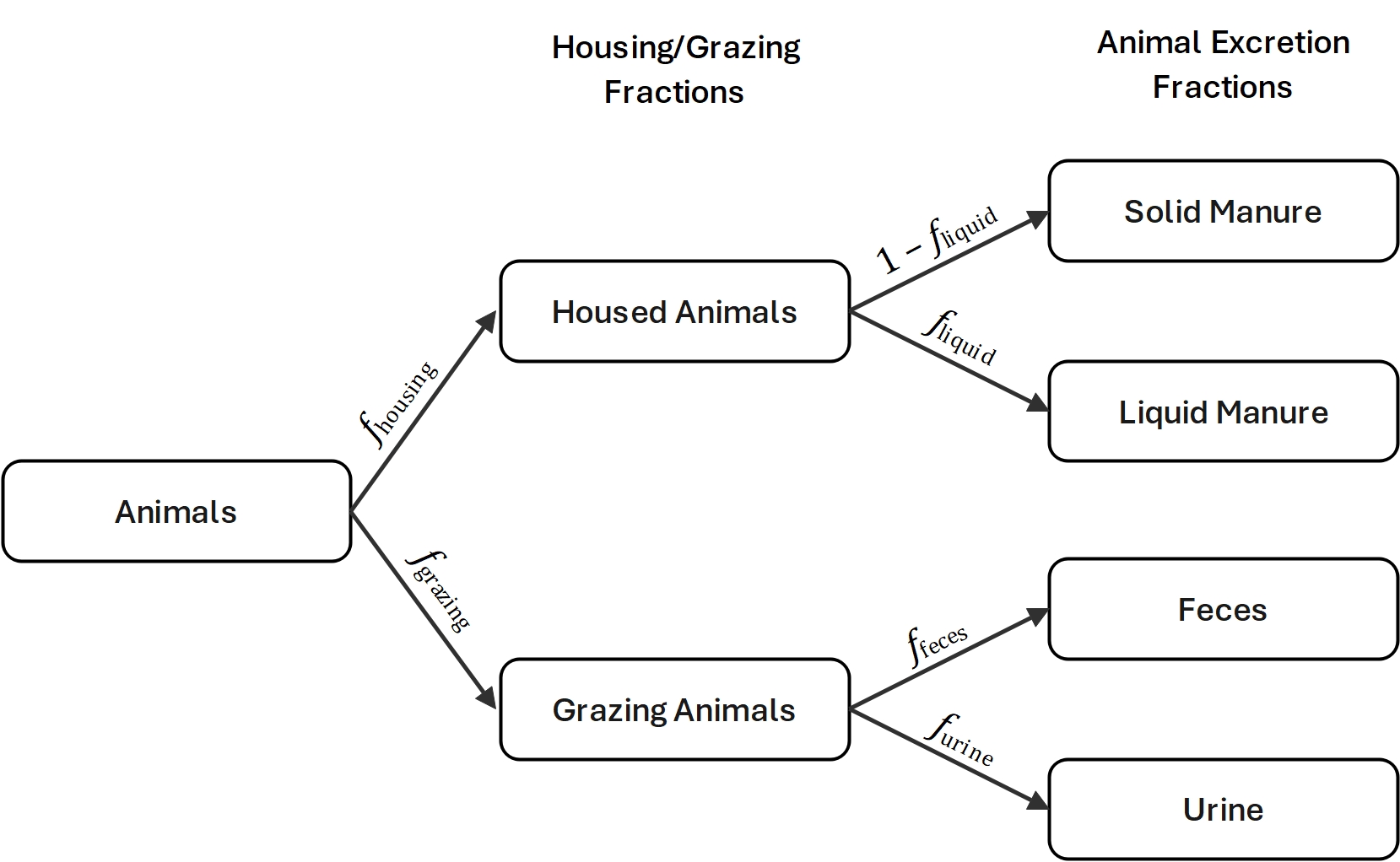
3. Livestock & Manure Management
Manure management systems
In Miterra, four types of manure management systems (MMS) are defined:
-
Housing
-
Farmyard
-
Storage: the storage of manure in unconfined piles/stacks, or in tanks/ponds/lagoons, typically for a period of several months to less than a year, before the manure may be applied to the field as fertilisers;
-
Grazing: the dung and urine deposited directly to the soil by grazing animals during grazing period.
The fractions of N excretions in each MMS (fhousing/yard/grazing) are derivd from IPCC NIRs ( Greenhouse Gas Inventory Data - Flexible queries Annex I Parties).
For each MMS, livestock excretions are handled in both solid and liquid forms. The respective fractions of solid and liquid manure are determined by a predefined liquid-solid manure collection parameter (fliquid), which is specific to region and animal type.
N content in livestock excretion
N content in livestock excretion is calculated for each type of animal and each type of excretion (solid or liquid):
where:
|
is the average amount of N in excretion that a single animal produces in one year (kg N head–1 year–1). |
|
|
is the fraction of N excreted during housing, farmyard, or grazing period. |
|
|
is the fraction of solid or liquid manure collected for the livestock in a region. |
CH4 emissions
CH4 emissions originates from enteric fermentations, and manure methanogenesis during manure storage, and are calculated on the basis of animal numbers.
where:
|
is the emission factor of CH4 for enteric fermentation, or manure storage (kg CH4 head–1 year–1). |
4. N Emissions from Manure Management
In this section, N emissions from livestock housing, farmyard, and manure storage are calculated. N emissions during field application of manure, and during grazing period are calculated in 10. N Losses from Soil when they are added to the soil.
Emissions of N are calculated separately for each type of animal, and for both solid and liquid forms, in each MMS. Unless otherwise specified, the units for all N terms are kg N ha–1 yr–1. The following table summarises the pathways for N emissions and losses calculated in this section.
| Housing | Yard | Storage | |
|---|---|---|---|
NH3 |
✅ |
✅ |
✅ |
N2O |
✅ |
||
NOx |
✅ |
✅ |
|
N2 |
✅ |
||
Loss to water [1] |
✅ |
[1] Includes combined runoff and leaching during manure storage.
NH3-N emissions are calculated on the basis of total ammoniacal N (TAN), following the approach by the EMEP/EEA air pollutant emission inventory guidebook 2023 (hereafter “EMEP Guidebook 2023”), with some simplification due to limitation on data availability. All the other gaseous N emissions are calculated based on total N.
The amounts of total N in solid and liquid forms of each type of animal manure in each stage are determined following the steps as described in N content in livestock excretion.
| Solid | Liquid | |
|---|---|---|
Housing |
Nhousing, soli |
Nhousing, liquid |
Farmyard |
Nyard, solid |
Nyard, liquid |
Grazing |
Ngrazing, solid |
Ngrazing, liquid |
Next, the amounts of TAN deposited during housing, yard, and grazing period, are calculated by multiplying N content with TAN fraction:
| Livestock Manure | fTAN | Ehousing | Eyard | Estorage | Eapplication | Egrazing |
|---|---|---|---|---|---|---|
Dairy cattle |
0.6 |
0.08 |
0.30 |
0.32 |
0.68 |
0.14 |
Non-dairy cattle |
0.6 |
0.08 |
0.53 |
0.32 |
0.68 |
0.14 |
Finishing pigs |
0.7 |
0.23 |
0.53 |
0.29 |
0.45 |
|
Sows & piglets |
0.7 |
0.24 |
0.29 |
0.45 |
||
Sheep |
0.5 |
0.22 |
0.75 |
0.32 |
0.90 |
0.09 |
Goats |
0.5 |
0.22 |
0.75 |
0.28 |
0.90 |
0.09 |
Horses |
0.6 |
0.22 |
0.35 |
0.90 |
0.35 |
|
Buffalo |
0.5 |
0.20 |
0.17 |
0.55 |
0.14 |
|
Laying hens |
0.7 |
0.20 |
0.08 |
0.45 |
||
Broilers |
0.7 |
0.21 |
0.30 |
0.38 |
||
Other poultry |
0.7 |
0.39 |
0.21 |
0.51 |
||
Other animals |
0.6 |
0.27 |
0.09 |
️ Reproduced from Table 3-9 of Chapter 3.B of the EMEP Guidebook 2023.
N Emissions from livestock housing
Emissions of NH3-N and NOx-N are calculated during livestock housing.
The NH3-N emissions during housing are calculated by multiplying TAN with corresponding emission factors:
where:
|
is the NH3-N emission factor as specified in Table 4.1. |
|
|
is the fraction of emission reduction by applying NH3 abatement technique i during housing phase. |
|
|
is the fraction of farms that adopted the NH3 abatement technique in the region. |
|
|
is the set of NH3 abatement techniques applied in the region (i ∈ n). |
The NOx-N emissions during housing are calculated similarly to NH3-N, but by multiplying total N with corresponding emission factors:
where:
|
is the NOx-N emission factor with a default value of 0.003 for all animal manure in all countries. |
The next step is only relevant to solid manure deposited in livestock houses. It acccounts for the addition of N in animal bedding in litter-based housing systems, and the consequent immobilisation of TAN in that bedding. Total N and TAN in solid manure are then removed from livestock housing (denoted by ex_housing subscript), and passed to storage system, subtracting the gaseous N emissions.
where:
|
is the mass of bedding straw added (kg fresh weight yr–1). |
|
|
is the immobilization coefficient with a default value of 0.0067 kg N kg–1 straw ( Kirchmann & Witter, 1989; and Webb & Misselbrook, 2004). |
|
|
is the mass of N in that bedding straw (kg N yr–1). |
Default values for length of housing period, annual straw use in litter-based manure management systems, and the N content of straw are given below. If the actual housing period deviates from the values in the table, the amounts of straw and straw N added should be adjusted proportionally to the actual housing days.
Livestock |
Housing Period |
Straw |
N Added in Straw |
|---|---|---|---|
Dairy cattle |
180 |
1500 |
6.0 |
Non-dairy cattle |
180 |
500 |
2.0 |
Pigs |
365 |
200 |
0.8 |
Sheep & goats |
30 |
20 |
0.08 |
Horses |
180 |
500 |
2.0 |
️️ Reproduced from Table 3-7 of Chapter 3.B of the EMEP Guidebook 2023.
N losses from manure storage
Emissions of NH3-N, N2O-N, NOx-N, N2-N, and NO3–-N losses to water are calculated for manure storage.
In the first step, the amounts of total N and TAN that are passed to storage system are calculated. It is assumed that all yard manure (both solid and liquid forms) are collected into the slurry storage system.
| This step simplifies the method in EMEP Guidebook by assuming that all manure are stored before application. Manures applied to fields directly from livestock housing, and manures (mainly slurries) used as feedstocks for digestion, are not considered due to lack of reliable estimation. |
For liquid slurry:
For solid manure:
The NH3-N emissions from storage are calculated by applying emission factors on TAN.
All other gaseous N emissions are calculated by applying emission factors on total N.
Part of the N may also be lost to water as NO3– during storage. This can take place via seepage through the bottom of the storage tank, or via overflow during precipitation.
where:
|
is the emission factor of leaching during storage (kg N per kg excreted N per year), which is specific to the type of manure and storage system.
[1] Assuming that some manure may be washed from the concrete floor to the surrounding soil. |
||||||||||||||||||||||||||||||
Finally, the amounts of total N and TAN remaining after storage (denoted by ex_storage subscript) are calculated. Total N and TAN in solid and liquid forms may be combined at this step.
where i ∈ {solid, liquid}, and j ∈ {NH3, N2O, NOx, N2}.
Total N and TAN remaining after storage (Nex_storage and TANex_storage) is applicable to the fields as organic fertilisers. The distribution of applicable manure N to different crops are described in 7. Fertilization.
5. Water Fluxes
This section describes the methods to estimate fractions of water fluxes that end up in surface runoff, or leached into soil. The approach was originally described by Velthof et al. (2009), and modified in Review and further differentiation of pedo-climatic zones in Europe (2011, pp 63–66).
Surface runoff
Surface runoff occurs when rainfall exceeds the maximum infiltration level of the soil. In the Miterra models, a maximum runoff factor is determined based on slope classification, and then the actual runoff fraction (Lrunoff) is estimated by applying a group of reduction factors.
where:
|
is the maximum runoff factor dependenent on slope.
[1] Slope Percentage = tan(Slope Degree) × 100. |
|||||||||||||||||
|
is a reduction factor for land use or crop.
|
|||||||||||||||||
|
is a reduction factor for precipitation surplus.
|
|||||||||||||||||
|
is a reduction factor for soil type/texture, which is based on the clay content of the soil.
|
|||||||||||||||||
|
is a reduction factor for the depth to rock.
[1] The threshold value of 25 cm should be used, but ESDB only reports this value in 40 cm intervals. |
|||||||||||||||||
For a heterogeneous region with n distinct subareas (e.g., a NUTS region with more than one land use type or soil texture class), reduction factor for the region is calculated as an area-weighed average of all subareas:
where:
|
is the reduction factor for the i-th subarea. |
|
|
is the fraction of the i-th subarea to the total (agricultural) area of the region. |
Leaching
Similar to surface runoff, leaching fraction is estimated by applying a group of reduction factors to a theoretical maximum leaching.
where:
|
is the maximum leaching factor per soil texture type, which are based on ESDB “Dominant surface textural class” (database field
|
||||||||||||||||||||||
|
is a reduction factor for land use. It has a fixed value of 0.36 for grassland, and 1.0 for other land use. |
||||||||||||||||||||||
|
is a reduction factor for precipitation surplus, which differs per soil texture class (see Miterra texture class above).
|
||||||||||||||||||||||
|
is a reduction factor for average annual temperature.
|
||||||||||||||||||||||
|
is a reduction factor for maximum rooting depth. Rooting depth data are based on ESDB “Depth class of an obstacle to roots” (database field
|
||||||||||||||||||||||
|
is a reduction factor for soil organic carbon content. SOC data are based on ESDB “Topsoil organic carbon content” (database field
|
||||||||||||||||||||||
| For a heterogeneous region, reduction factors are calculated as area-weighed averages ( Equation 5.2). |
6. Crop Production
Harvested products
Yields of harvested products are provided as input. In Miterra, fresh yields are used for most crops except for grass (which uses dry matter yields), and then dry matter (DM) yields are simply calculated using a DM fraction for each type of crop.
N content in harvested products (Nharvest) is calculated using an N:DM ratio.
where:
|
is the fresh weight yield of the harvested crop product (kg fresh weight ha–1). |
|
|
is the average fraction of dry matter weight in the product (kg DM kg–1 fresh weight). |
|
|
is the fraction of total N in harvested dry matter (kg N kg–1 DM). |
For other nutrient elements (P, Ca, Mg, K, Na, Cl & S), the content in harvested products is calculated in the same way as N:
where:
|
is the fraction of element x in harvested dry matter (kg X kg–1 DM). |
For heavy metal elements (Cd, Cu, Pb & Zn), their content are calculated based on bioconcentration factors (BCF):
where:
|
is the content of element X in the soil (kg X ha–1). |
|
|
is the BCF of element x. |
Cover crops
Cover crop area
The areas of crops growing in the winter are determined for each crop type:
-
For winter wheat & winter barley, they are explicitly known as winter crops and their areas are available from input.
-
For soft wheat, durum wheat, barley, and rye, they can be grown either in spring or winter, and their areas of winter growth is determiend with a “winter share” fraction (fw).
Based on that we can estimate the areas of non-winter (spring) growth for each crop:
For each crop i in the region:
where:
|
is the area of crop i growing in the spring (ha). |
|
|
is the total area of the crop i (ha). |
|
|
is the fraction of crop i that is growing in the winter. Data are available from SoilCare (Eurostat/Corine). |
The area of cover crop growing after each crop is then estimated as:
For each crop i in the region:
where:
|
is the area of cover crop growing after crop i. |
|
|
is the total area of cover crops in the region. Data are available from Eurostat. |
The fraction of cover crop after each crop (fcc) is calculated as:
For each crop i in the region:
where:
|
is the area of crop i. |
Cover crop C and N production
The N uptake by cover crops is based on data from Schroder et al., who provided estimates per environmental zone on the N yield of cover crops based on temperature sum values. However, especially for Mediterranean climates these values seem high and there might be limitation by water and nitrogen. Therefore, the N uptake by catch crops is maximised at 75% of the soil N surplus, and a minimum value of 5 kg N ha–1 is applied as well. Previously a default value of 42 kg N ha–1 was used based on an average C input of 1500 kg ha–1 and a C:N ratio of 35, which is probably too high for most regions.
For each crop i in the region:
where:
|
is the N uptake by the cover crop following crop i, specific to the environmental zones.
|
||||||||||||||||||||||||||||||||||||||||
|
is the soil N surplus for crop i. Nsurplus is derived by running the model for initialization assuming no cover crops, and using the output on soil N surplus as input for future runs. |
The C content in cover crops is determined by assuming a C:N ratio of 25.
For each crop i in the region:
Residue removal & incorporation
For annual crops, part of the unharvested residue biomass may be further removed from the field (e.g., straw), and the rest may be incorporated into soil by tillage.
The biomass of unharvested residues, removed residues, and residues incorporated into soil, are calculated using different approaches for annual crops, straw crops, and perennial crops.
| In all calculations in this section, the fraction of C content in crop organic matter (fC) is assumed to be 0.45 for all crop types. |
Annual crops & grasslands
Most arable crops, except for straw crops (see below), are considered annual crops. The unharvested residues are calculated based on crop yields and harvest index.
Residue removal and incorporation for grasslands are calculated in the same way as annual crops.
where:
|
is the harvest index, which is the ratio of harvested biomass to the annual net primary production. |
|
|
is the ratio of N in harvested products to N in residues. |
The amount of residues removed from the field is determined by a country- and crop-specific removal factor.
where:
|
is the fraction of crop residues removed from field. |
Straw crops
Straw crops include cereal crops, maize, rice, sunflower, and rapeseed. Carbon inputs to soil from straw crops consist of aboveground (Cabove) and belowground residues (Cbelow). The aboveground residue biomass (Mabove) is calculated according to Scarlat et al. (2010):
where:
|
is the fresh weight yield of the harvested crop product (kg ha–1). |
||||||||||||||||||||||||||||
|
are crop-dependent regression parameters.
|
The aboveground residue biomass is split into stubble (0.45) and straw (0.55). A fraction of the straw is removed, and the remaining part is incorporated into soil along with the stubble. The total C incorporation from aboveground residues is thus calculated as:
where:
|
is the removal fraction of straw. |
|||||||||||||
|
is the fraction of dry matter in the stubble and straw.
|
The belowground residue C is always considered as incorporated, and is calculated according to Taghizadeh-Toosi et al. (2014):
where:
|
is the fresh weight yield of the harvested crop product (kg ha–1). |
|
|
is the fraction of dry matter in the product. |
|
|
is the biomass of aboveground residues (kg ha–1). |
|
|
is the fraction of dry matter in the stubble and straw. |
|
|
is the ratio of root biomass and exudate C (below-ground C) of total net C assimilation, with a default value of 0.25. |
The amount of N in residues removed and incorporated into soil for straw crops is calculated as:
where:
|
is the fraction of N in stubble and straw dry matter. |
Perennial crops
Perennial crops include fruit trees, olive trees, and grapes. Residue inputs from these crops consist of pruned leaves, dead leaves, fruit losses during growth and harvest, dead roots, root exudates, and input from grass cover.
- Pruned residues
-
Yields for pruned branches and leaves are available for rainfed and irrigated fields. Part of the pruned biomass is removed, and the rest incorporated.
Equation 6.15where:
is the pruning potential for irrigated land (kg DM ha–1 yr–1).
is the pruning potential for rainfed land (kg DM ha–1 yr–1).
is the fraction of area under irrigation.
is the fraction of pruned biomass that is removed from field.
is the C:N ratio of prunnings, with a default value of 60.
- Leaf litters
-
Include input from dead leaves.
Equation 6.16where:
is the dry matter yield of the harvested crop product (kg ha–1. Equation 6.1).
is the ratio of leaf to fruit biomass.
is the C:N ratio of leaf litters, with a default value of 30.
- Dead fruits
-
Include input from fruit losses during growth and harvest.
Equation 6.17where:
is the fraction of yield biomass lost during growth.
is the fraction of yield biomass lost during harvest.
is the fraction of total N in harvested fruit dry matter (kg N kg–1 DM).
- Belowground residues
-
Include dead roots and root exudates.
Equation 6.18where:
is the ratio of rhizodeposition to fruit biomass.
It is assumed that the fine root biomass is the same as root exudates, therefore the left term is multiplied by 2 to give total belowground C input.
is the C:N ratio of roots and root exudates, with a default value of 30.
- Total C input to soil
-
Equation 6.19
- Total N input to soil
-
Equation 6.20
- Additional residues from soil cover
-
The grounds of some orchards are covered by grass, which contribute additionally to soil C and N input:
Equation 6.21where:
is the dry matter yields of permanent grassland in the region (kg DM ha–1).
it is assumed that grass cover yield is half of the yield of normal grassland.
is the fraction of area covered by grass in the orchard.
is the C:N ratio in grass residues with a default value of 20.
Cover crops
In case cover crops are grown, more crop residues will be available. It is assumed that all cover crops are incorporated into soil. The amounts of cover crop N and C incorporated into soil are calculated by Equation 6.7 and Equation 6.8, respectively.
Other lands
For fallow and set-aside lands, which are not cultivated but may have growth of weeds, it is assumed that 250 and 500 kg C ha–1, respectively, are incorporated into soil annually. The C:N ratio of the incorporated residues is assumed to be 30.
Removal and incorporation of other elements
Removal and incorporation of other elements (P, Ca, Mg, K, Na, Cl, S, Cd, Cu, Pb, and Zn) is only calculated for straw crops. The amount removed/incorporated is based on the N removed/incorporated and N:X ratios.
where:
|
is the content of element X in removed/incorporated residues (kg X ha–1). |
|
|
is the N content in removed/incorporated residues (kg N ha–1). |
|
|
is the N:X ratio of the residue. |
Crop uptake & demand
Crop N uptake is simply calculated as the total N content in both harvested products and unharvested biomass.
Crop demand refers to the rate of N fertilization required to satisfy crop uptake. Since not all N in the soil may become available to crops, a higher rate of N than crop uptake must be applied. This is determined by an uptake efficiency factor.
where:
|
is the crop uptake efficiency factor.
|
Biological N fixation
Miterra uses a simple, static approach to estimate N fixation by assigning fixed N amounts to different crops. The table below gives the default values assumed by Miterra.
| Crop Type | N Fixation |
|---|---|
Soybeans |
80% of Nuptake. |
Pulses |
70% of Nuptake. |
Arable & perennial crops |
2 kg N ha–1 yr–1 |
Grassland |
7.5 kg N ha–1 yr–1, assuming no grass-clover mixture. |
7. Fertilization
This section describes an approach to apply local derogation and distribute N fertilisers to various crops within a country. This distribution is mostly relevant to Miterra-Europe, as information on application rates to different crops is often lacking. For Miterra-Farm, fertiliser application rate to each crop should be provided as an input. However, if such data is not available, the method below may also be used.
Distribution of grazing excretions
Animal excretions during grazing are distributed to permanent grasslands, temporary grasslands and rough grazings (natural grasslands). It is assumed that all permanent grasslands are used for grazing, half of the temporal grasslands are used for grazing (because they are often used for mowing/silage), and the grazing intensity on natural grasslands is 50% lower than on permanent grasslands (equivalent to half of the natural grasslands are grazed). The deposition rate of grazing excretion (kg N ha–1) is therefore calculated as follows:
where:
|
represents permanent, temporary, and natural grasslands, respectively. |
|
|
is the total N in solid and liquid excretions during grazing in the region (kg N). |
|
|
is the area of respective grassland type (ha). |
Distribution of animal manure
Animal manure is distributed based on both manure type and crop type, following the approach described by Gerard et al. (2009).
| Manure Type | Crop Type | Distribution |
|---|---|---|
Cattle, sheep & goat manure |
Fodder crops |
Each type of manure is evenly distributed to all fodder crops. |
Pig manure |
Fodder crops |
25–75% of total manure N remaining after storage, distributed to all fodder crops in equal amount per hectare.
|
Group I crop |
Receives the remaining 75–25% of manure N; distributed as follows:
|
|
Group II crop |
||
Group III crop |
||
Poultry manure |
Non-fodder crops |
Distributed among all non-fodder crops in equal amount per hectare. |
Derogation & redistribution of manure N
EU Nitrates Derective sets a maximum rate of 170 kg N ha–1 for manure application, unless local derogations apply. The manure N application rate must not exceed the maximum rate, and if it does, the extra manure may be reallocated to other crops in the region or country.
Step 1
The maximum manure N allowed (Nmax), and the provisionally applied manure N (Napp) are calculated for each crop in each region of the country:
where:
|
is the maximum manure N rate (kg N ha–1) allowed for crop c in region r by EU Nitrates Directive or local derogation. |
|
|
is the N application rate (kg N ha–1) of manure type m for crop c in region r, as estimated in Distribution of animal manure. |
|
|
is the area of crop c in region r (ha). |
To disaggregate Napp[r, c] among each manure type later, λ[r, m] is the ratio of N in manure type m to the total manure N applied in region r.
Step 2
The manure N surplus and gap is determined for each crop in each region:
If :
Else:
Step 4
4.1: If Nsurplus, country = 0: There is no surplus in the country (i.e., every crop in every rgion received no more manure N than what’s permitted by regulation). No derogation or redistribution is available in this case.
4.2: If Nsurplus, country > 0: There is a surplus in the country, which may be redistributed to crops with a gap in the country. We consider 2 scenarios:
4.2.1: If Nsurplus, country ≥ Ngap, country: There is enough surplus in the country to cover the gap in all regions of all crops.
4.2.2: If Nsurplus_country < Ngap_country: There is a surplus in the country, but it is not sufficient to cover all the gaps. A proportion of the country surplus is redistributed, which is equal to the relative size of the regional deficit to the country deficit.
If :
Else:
| Since Nsurplus, country < Ngap, country, the right-hand side will never exceed Nmax. |
Manure export
The amount of manure N transported out of the country is calculated by comparing the total amount applied before and after derogtion/re-distribution. Any manure that is not field applied is assumed to be exported. No destination for manure export is assumed: manures are not tracked by the Miterra model once they are transported out of the country border.
where:
|
is the total amount of manure N applied (kg N) for crop c in region r before derogation/re-distribution. |
|
|
is the total amount of manure N applied (kg N) for crop c in region r after derogation/re-distribution. |
Crop available N
The plant available N (Navail) is calculated from applied manure, grazing excretion, deposition and crop residues. This value is then be substracted from the crop N demand to give a more realistic mineral fertilizer application per crop.
The plant available N is calculated in two parts: Navail, mineral for mineral N sources, and Navail, organic for N mineralized from crop residues, and organic fractions of manure & grazing excretions. The total Navail is the sum of the two parts.
Crop available N from mineral N sources
where:
|
is the total mineral N from applied manure (kg N ha–1. See Distribution of animal manure). If mineral N fraction is unknown, the default value is assumed to be 0.75 for solid manure, and 0.4 for liquid slurry. |
||||||||||||||||||
|
is the total mineral N from grazing excretions (kg N ha–1. See Distribution of grazing excretions). If mineral N fraction is unknown, the default value is assumed to be 0.5. |
||||||||||||||||||
|
is the total N from compost (kg N ha–1. See Nutrient content in compost). |
||||||||||||||||||
|
is the total N from sludge (kg N ha–1. See Nutrient content in sludge). |
||||||||||||||||||
|
is the annual N input from atmospheric deposition (kg N ha–1). |
||||||||||||||||||
|
are coefficients for plant available N for the respective N source.
|
Crop available N from organic N sources
where:
|
is the amount of N in inccorporated crop residues (kg N–1 ha, see Residue removal & incorporation). |
|
|
is the amount N uptake by cover crops following the main crop (kg N–1 ha, see Cover crop C and N production). |
|
|
is the area fraction of cover crops following the main crop (see Equation 6.6). |
|
|
is the fraction of mineralized N that is available to crops, with a default value of 0.9 for grasslands, and 0.7 for other crops. |
Finally, the total plant available N is determined by combining the two parts above:
Distribution of mineral N fertilisers
First, the requirement of mineral N fertilisers by each crop (Nreq) is determined from crop N demand and N already available to the crop from other sources. To obtain a more equal fertiliser distribution among crops, we assume that at least 30% of the N demand will come from mineral fertiliser.
where:
|
is the N demand by the crop (kg N–1 ha. See Equation 6.24). |
|
|
is the soil available N to the crop (kg N–1 ha). |
The mineral N fertilizers are distributed over crops using weighing factors, so that crop with highest N demand receives the highest amount of N fertilizers. The weighing factors are calculated from the crop N uptake and the total area of the crop.
For crop i in the region:
where:
|
is the weighing factor for the crop. |
|
|
is the total area of the crop in the region (ha). |
|
|
is the collection of all crops grown in that region, i ∈ n. |
|
|
is the application rate of mineral N fertilisers for the crop (kg N ha–1). |
|
|
is the sum of the amount of all types of mineral N fertiliser applied in the region (kg N). |
8. Compost & Sludge
Estimation of compost and sludge application
Based on Saveyn & Eder (2013), it is assumed that on average 51% of the compost produced is used in agriculture, and the rest is used in public green, gardening, and horticulture. Compost is assumed to be distributed evenly to all crops except grassland.
For sludge, the amount used for agriculture in each EU member state is provided as input (data source: Eurostat, 2020). Sludge is distributed evenly to all crops except grassland.
Nutrient content in compost
Nutrient content in compost is calculated based on the composition of the compost product ( Regelink et al., 2021). All values are given in g kg–1.
| Compost Type | DM | C | N | P | K |
|---|---|---|---|---|---|
Biowaste |
620 |
114.2 |
7.9 |
1.66 |
4.9 |
Greenwaste |
649 |
145.1 |
4.9 |
0.96 |
5.6 |
According to Geisseler et al. (2021), on average 16-17% of total N was present as mineral N in various organic fertilizers and composts. It is therefore assumed that 16% of the total N in compost is in inorganic form, and the rest is organic.
Nutrient content in sludge
Based on Driessen & Roos (1996), the following assumptions are made on the composition of sludge:
-
The average and median organic matter content is ca. 50%.
-
C content is assumed to be 50% of organic matter.
-
For N, the average and median N content is ca. 44 g kg–1 .
-
For P, the content is country-specific, ranging from 0.9% to 6.7%, with an average of 3.3%.
-
For K, the average and median K content is ca. 8 g kg–1 DM.
Similar to compost, it is assumed that 16% of the sludge N is inorganic, and the rest is organic.
9. Input To & Output From Soil
This chapter summarises how to calculate the input of different (nutrient) elements to soil.
Input to soil
C input
- From crop residues
-
Organic C content in crop residues incorporated into soil is described in Residue removal & incorporation.
- From manure
-
C inputs from manure application and grazing excretions are estimated based on manure N content and manure C:N ratio. As a safety check to prevent unrealistic high values, C input from grazing excretions is capped at 2500 kg C ha–1 year–1.
- From compost & sludge
-
C inputs from compost and sludge are described in 8. Compost & Sludge.
N input
External N input sources to soil include mineral N fertilisers, manure application, grazing excretion (grassland only), compost, sludge, atmospheric deposition, and biological N fixation. The total amount of N input varies depending on crop and region.
where:
|
is the total N content in mineral fertilisers applied to the field (see Distribution of mineral N fertilisers]). |
|||
|
is the total N content in manure applied to the field (see Distribution of animal manure). |
|||
|
is the total N content in urine and feces excreted during grazing (only for grasslands; see Distribution of grazing excretions). |
|||
|
is the total N content in compost applied to the field (see Nutrient content in compost). |
|||
|
is the total N content in sludge applied to the field (see Nutrient content in sludge). |
|||
|
is the total atmospheric NH3 and NOx depositions to the field, which are part of default Miterra input derived from regional deposition maps. |
|||
|
is the biologically fixated N, as calculated in Biological N fixation.
|
P input
- From atmospheric deposition
-
At present the deposition map is not updated to the input data yet. Currently, P deposition of 1 kg P ha–1 year–1 is assumed.
- From mineral fertilisers
-
P input from mineral fertilisers are calculated based on the application rate of each type of fertiliser, and the P content in the fertiliser.
- From manure
-
P content in applied manure and grazing excretions are estimated based on N content and N:P ratios of the manure.
- From compost & sludge
-
P inputs from compost and sludge are described in 8. Compost & Sludge.
Input of other elements
Other elements include Ca, Mg, K, Na, Cl, S, Cd, Cu, and Zn. Not all elements are accounted for in each input source.
- From atmospheric deposition
-
Atmospheric depositions of Ca, Mg, K, Na, S, Cd, Cu, and Zn are available as part of Miterra default database.
- From mineral fertilisers
-
Element inputs from mineral fertilisers are calculated based on the application rate of each type of fertiliser, and the composition of the fertiliser.
- From manure
-
Input of other elements to soil from manure is estimated based on the total manure N applied, and the corresponding N:X ratio in manure, where X may be Ca, Mg, K, Na, Cl, S, Cd, Cu, or Zn.
Equation 9.2where
is the content of element X in applied manure (kg X ha–1);
is the N content in applied manure (kg N ha–1); and
is the N:X ratio of applied manure.
- From compost & sludge
-
Input of K are calculated for compost and sludge, as described in 8. Compost & Sludge.
Output from soil
C output
Emission of CO2 is the only C output pathway from soil, which is modelled by RothCN (see Decomposition of organic carbon).
N output
N output pathways include:
-
Harvest of crop products (see Harvested products);
-
Removal of crop residues (see Residue removal & incorporation);
-
Emissions to the environment in the forms of N gases, surface runoff, and leaching (see 10. N Losses from Soil).
P output
P output pathways include:
-
Harvest of crop products (see Harvested products);
-
Removal of crop residues (see Residue removal & incorporation);
-
Loss to water via surface runoff and leaching (see Runoff and leaching).
Output of other elements
Output pathways for other elements include:
-
Harvest of crop products (see Harvested products);
-
Removal of crop residues (see Removal and incorporation of other elements);
-
Loss to water via surface runoff and leaching.
-
For S, see Runoff & leaching.
-
For heavy metal elements (Cd, Cu & Zn), see Runoff & leaching.
-
For Ca, Mg, K, and Na, see Runoff and leaching.
-
10. N Losses from Soil
Part of the N applied to the soil is lost in forms of gaseous emissions, including NH3, N2O, and NOx, as well as surface runoff and leaching. The following table summarizes the emissions from different sources that are calculated in the Miterra models.
| Mineral Fertilisers | Manure Application | Grazing Excretion | Crop Residues | |
|---|---|---|---|---|
NH3 |
✅ |
✅ |
✅ |
|
N2O |
✅ |
✅ |
✅ |
✅ |
NOx |
✅ |
✅ |
✅ |
|
Surface Runoff |
✅ |
✅ |
✅ |
|
Leaching [1] |
✅ |
|||
NH3 volatilization
For solid manure applied to the field or deposited during grazing, NH3-N volatilization is calculated as a fraction of the TAN applied. For mineral N fertilisers, NH3-N emissions depends on total N applied and soil pH.
For mineral N fertilisers:
For manure:
where:
|
is the amount of total N applied to the soil in mineral N fertilisers. |
|||||||||||||||||||||||||||||||||||||
|
is the amount of TAN applied to the soil in manures or grazing excretion. |
|||||||||||||||||||||||||||||||||||||
|
is the specific NH3 emission factor which differs depending on the TAN source. Mineral N fertilisers
️ Reproduced from Table 3-2 of Chapter 3.D of the EMEP Guidebook 2023. Solid manure |
Liquid slurry
For liquid slurry, NH3-N emissions are estimated using the ALFAM2 model, which adopts a more dynamic approach taking into account slurry composition, climate, and application method.
N2O emissions
N2O emissions are calculated using EFs following the 2019 IPCC Guidelines.
where:
|
is the total N content in mineral N fertilisers, manures, grazing excretion, or crop residues. |
||||||||||||||||||||||||||||||||||||||||||||||
|
is the N2O emission factor which differs depending on climate zones and N sources.
The climate zones are determined based on annual average temperature (T), annual total precipitation (P) and annual total evapotranspiration (E).
|
NOx emissions
Emission factor for NOx is linked to annual precipitation amount.
where:
|
is the total N content in mineral N fertilisers, manures, or grazing excretion. |
|||||||||||||||
|
is the NOx emission factor which differs depending on the annual precipitation of the region.
|
Surface runoff of N
N loss via surface runoff is calculated using a runoff fraction:
where:
|
is the total N content in mineral N fertilisers, manures, or grazing excretion. |
|
|
is the runoff fraction of precipitation surplus, which is calculated in Surface runoff. |
N surplus
Three types of N surpluses are defined in Miterra:
- Gross N surplus
-
is the difference between gross N input and crop N removal (both by harvest and residue removal) at farm level:
Equation 10.5where:
is the total N in livestock excretion produced at farm level or in the region (see N content in livestock excretion).
is the total N removed by harvest and residue removal at farm level or in the region (see Residue removal & incorporation).
- Soil N surplus
-
is the difference between soil N addition and crop N removal at field level. Soil N surplus is an indicator for the potential of N losses to the environment.
Equation 10.6 - Corrected soil N surplus
-
is the difference between soil N addition and soil N losses, including gaseous emissions, surface runoff, and crop removal, at field level. Corrected soil N surplus reflects the potential for N leaching and denitrification.
Equation 10.7
N leaching
The Miterra models assume that there is no change in the soil mineral N pool, and that all N applied to the soil which is not lost at soil surface, nor taken up by the crop, are either leached below root zone, or lost to the atmosphere via denitirfication.
N leaching may be determined in two parallel approaches:
- Method 1: Coventional Miterra Approach
-
Leaching is a fraction of the corrected soil total N surplus (i.e., the organic and mineral N fractions are lumped) as described in Equation 10.7.
- Method 2: The RothCN Approach
-
The RothCN model calculates changes in soil mineral N pool as the balance of mineralization and immobolization during soil organic matter decomposition. Leaching is then estimated as a fraction of corrected soil mineral N surplus (See Emissions and balances).
where:
|
is the fraction of precipitation surplus leached below the root zone, which is calculated in Leaching. |
| Due to the nature of approximate estimation in Miterra, the calculated Nsurplus, corrected may be < 0. In that case, Nsurplus_corrected, leaching, and denitrification should all be set to 0 to avoid negative values. |
The N that has leached below root zones are further partitioned to leaching to groundwater, and interflow that end up in large surface waters, which are determined by a ground flow fraction ( ). The ground flow fraction is a region-specific coefficient based on the modelling by Keuskamp et al. (2012).
The part of N(surplus, corrected) that is not leached, is denitrified.
11. Soil P Dynamics
Apart from input and uptake, the P concentration in the topsoil and subsoil is affected by P accumulation. Modelling of P accumulation or release is included by using a Langmuir equilibrium, supplemented with rate limited diffusion, based on the approach used in the INITIATOR model (van der Salm et al., 2016#; #De Vries et al., 2023).
Division of pools
The soil P pool is divided into:
-
An inert P pool with no change over time,
-
A stable P pool, S, changing slowly according to a rate limited reaction with dissolved P in the soil solution, and
-
A labile P pool, L, changing rapidly according to an equilibrium reaction with dissolved P in soil solution.
Initialization
The sum of the labile and stable pool is assumed to be approximated by oxalate extractable P (Pox), further denoted as the reactive P pool. The initial size of Pox must be provided by user. The labile pool, L, is at the start assumed to be 1/3 of Pox, and the stable pool, S, thus being equal to 2/3 of Pox.
The maximum size of Pox is assumed to be 1/2 of (Al + Fe)ox, with (Al + Fe)ox being the oxalate extractable Al and Fe contents (mmol kg–1).
Soil P concentrations
The concentration of inorganic P in soil solution, [Pi], is calculated from the size of the labile P pool (L) according to a Langmuir equation:
where:
|
is the size of the adsorbed labile P pool (mmol kg–1). |
||||||||||||||||
|
is the theoretical maximum adsorption (mmol kg–1), which is 1/6 of (Al+Fe)ox. |
||||||||||||||||
|
is a Langmuir adsorption constant (m3 kg–1).
|
||||||||||||||||
|
is the inorganic P concentration (g m–3, or mg L–1). The value of 1000 is used to convert result from kg m–3 to g m–3 (mg L–1). |
If any calculated value falls outside the boundaries, the value must be clipped. See Minimum and maximum pool sizes for further explanation. |
The total (both inorganic and organic) P concentration, Pt, is then derived using an exponential relationship between total P and inorganic P based on measurements in soil solution, drainage water and surface water, as reported by Chardon et al. (2007) (in Dutch):
where:
|
is the total P concentration (g m–3, or mg L–1). |
|
|
is the inorganic P concentration (g m–3, or mg L–1). |
The transfer between P in the soil solution and the stable pool, Ptrans, is described by a rate-limited Freundlich equation:
where:
|
is the rate constant (day–1) for the transfer from soil solution to the stable pool, with a default value of 0.0014. |
|
|
is the rate constant (day–1) for the transfer from the stable pool to soil solution, with a default value of 2 × 10⁻⁶ for sand, and 44 × 10–6 for clay and peat soils. |
|
|
is the Freundlich constant of the stable pool (mmol kg–1 (mg L–1)–n).
|
|
|
is the inorganic P concentration (g m–3, or mg L–1). |
|
|
is the exponent of stable pool, with a default value of 0.26. |
|
|
is the size of the stable pool (mmol kg–1). |
|
The value of Ptrans can be positive or negative. When Ptrans > 0, dissolved P transfers to S; and when Ptrans < 0, S transfers to dissolved P. |
P surplus
P surplus is simply calculated as the difference between P input and crop P uptake:
where:
|
is the annual P deposition (kg P ha–1 yr–1). |
|
|
is the annual P input from mineral fertilisers (kg P ha–1 yr–1). |
|
|
is the annual P input from animal manure (kg P ha–1 yr–1). |
|
|
is the annual P removed from soil by crop uptake (kg P ha–1 yr–1). |
Runoff and leaching
P runoff and leaching are calculated based on the total P concentration and the waterflux:
where:
|
is the total P concentration (g m–3, or mg L–1). |
|
|
is the daily interflow (subsurface runoff) (m3 ha–1 day–1). |
|
|
is the daily leaching effluent to shallow groundwater (m3 ha–1 day–1). |
| For calculations of Qint and Qeff, refer to 5. Water Fluxes. |
P accumulation
P accumulation (Pacc) is calculated as:
where:
|
the P surplus (g ha–1 day–1). |
|
|
is the loss of P by leaching and runoff (g ha–1 day–1). |
Pool dynamics
The changes in the labile and stable pools are calculated on a daily basis.
The change in the labile P pool is calculated by a mass balance:
where:
|
are the size of the labile P pool (mmol kg–1) at time t + 1 and time t, respectively. |
|
|
is the P accumulation (g ha–1 day–1). |
|
|
is the transfer flux from the soil solution to the stable pool of adsorbed P (mmol kg–1 day–1). |
|
|
is the length of the time step (1 day). |
|
To convert the unit of and from g ha–1 day–1 to mmol kg–1 day–1: where:
|
The change in the stable P pool is calculated as:
where:
|
are the size of the stable P pool (mmol kg–1) at time t + 1 and time t, respectively. |
|
|
is the transfer flux from the soil solution to the stable pool of adsorbed P (mmol kg–1 day–1). |
|
|
is the length of the time step (1 day). |
The change in the reactive P pool, Pox, can be determined as:
Minimum and maximum pool sizes
From Equation 11.2 it can be deduced that when L approaches L'max, [Pi] can become infinitely high. To maintain [Pi] in a reasonable range, we set for [Pi] a minimum value of 0.001 mg L–1, and a maximum value of 90 mg L–1.
The minimum and maximum boundaries Lmin and Lmax may be determined as:
The upper boundary of S pool is equal to Smax, which is defined as:
The calculated size of L and S in each time step is checked so that they do not exceed the boundaries:
Buffer pool for excess P
Following Equation 11.13, in the case of Lt > Lmax or St > Smax, Lt and St are clipped to their respective maximums. The excess P (Lt − Lmax or St − Smax) must go to a provisional buffer pool B, which acts as a precipitation pool to temporarily store these excess P.
The buffer pool also have precedence over L and S in P mining. When B > 0, any transfer of adsporped P to soil solution will first come from B, and any remainder will then come from L and S.
The following pseudocode in Python demonstrates how the buffer pool is used. The dynamics of S is calculated before the dynamics of L.
P_trans = ... # Transfer flow between dissolved P and adsorped stable P pool.
B = ... # Buffer precipitation pool.
dB = ... # Change in the B pool.
S = ... # Adsorped stable P pool.
S_max = ... # Maximum size of the S pool.
if P_trans < 0: (1)
if abs(P_trans) > B: (2)
dB = -B
P_trans = P_trans + B
else: (3)
dB = P_trans
P_trans = 0
else: (4)
if S + P_trans < S_max: (5)
dB = 0
else: (6)
dB = S + P_trans - S_max
(7)
B = B + dB
S = S + P_trans
S = min(S, S_max)| 1 | Transfer from adsorped stable pool to dissolved P. B is used before S. |
| 2 | B is smaller than Ptrans, B is depleted, and Ptrans is offset by B. |
| 3 | B is larger than Ptrans, Ptrans is set to 0 since no P will be coming from S, and B is reduced by Ptrans. |
| 4 | Transfer from dissolved P to adsorped stable pool. B acts as a buffer pool for excess P. |
| 5 | No excess P. B remains unchanged. |
| 6 | Excess P goes into B. No need to adjust the sizes of Ptrans or S, since S + Ptrans will be clipped to Smax. |
| 7 | Update the sizes of B and S. |
P_acc = ... # P accumulation.
P_trans = ... # Transfer flow between dissolved P and adsorped stable P pool.
B = ... # Buffer precipitation pool.
dB = ... # Change in the B pool.
L = ... # Adsorped labile P pool.
L_min = ... # Minimum size of the L pool.
L_max = ... # Maximum size of the L pool.
dL = P_acc - P_trans (1)
if dL < 0: (2)
if abs(dL) > B: (3)
dB = -B
dL = dL + B
else: (4)
dB = dL
dL = 0
else: (5)
_L = L + dL
if _L < L_min: (6)
if abs(_L - L_min) > B: (7)
dB = -B
else: (8)
dB = _L - L_min
elif _L > L_max: (9)
dB = _L - L_max
else: (10)
dB = 0
(11)
B = B + dB
L = L + dL
L = max(L_min, min(L, L_max))| 1 | Change in size of the L pool (ΔL) is determined according to Equation 11.8. |
| 2 | Ptrans > Pacc > 0, B is used before L. |
| 3 | B is smaller than ΔL, B is depleted, and ΔL is offset by B. |
| 4 | B is larger than ΔL, ΔL is set to 0 since no P will be coming from L, and B is reduced by ΔL. |
| 5 | Pacc > Ptrans and/or Ptrans < 0, and the size of L will increase to a provisional new size L'. |
| 6 | When L' < Lmin, L' will be padded to Lmin, and the difference ( |L' − Lmin| ) will come from B. |
| 7 | B is smaller than the difference, B is depleted. Note that in this case a small amount of P ( |L' − Lmin| − B ) will appear to be coming out of nowhere. However, since this value will be very small, it may be safely negelected. |
| 8 | B is larger than the difference, B is reduced by the amount of the difference. |
| 9 | When L' > Lmax, B acts as a buffer pool for excess P. |
| 10 | When Lmin < L' < Lmax, B remains unchanged. |
| 11 | Update the sizes of B and L. |
12. Soil S Dynamics
SO4 adsorption-desorption
SO4 accumulation or release is limited to an adsorption-desorption isotherm that governs the flux of SO4 between dissolved and sorbed phases. Unlike P, no distinction is made in stable and labile pools, thus not including a rate limited flux from a stable to a labile pool. SO4 adsorption-desorption is described by an extended Freundlich equation, with the inclusion of pH impacts on adsorption constant, according to Martinson et al.(2003), and Gustafsson et al. (2015):
where
|
is the amount of adsorbed SO4 (mol kg–1). |
|
|
is the Freundlich SO4 adsorption coefficient, with a default value of 2. |
|
|
is the total dissolved SO4 concentration (mol L–1). |
|
|
pH measured in MgCl2 or CaCl2. |
|
|
is the total dissolved proton (mol L–1). |
|
|
are Freundlich equation parameters, with a default value of m = 0.2 and n = 1.7. |
Initialization
The initial SO4 concentration in soil solution is calculated by assuming equilibrium with the historic S input and uptake in soils in the past:
where
|
is the initial concentration of SO4 in soil solution (mol L–1). |
|
|
is the historic average combined S input from all sources (kg ha–1yr–1). |
|
|
is the historic average S uptake (kg ha–1 yr–1). |
|
|
is the annual interflow (subsurface runoff) (m3 ha–1 yr–1). |
|
|
is the annual leaching effluent to groundwater (m3 ha–1 yr–1). |
|
|
is the molar mass of S (32 g mol–1). |
| For calculations of and , refer to 5. Water Fluxes. |
The initial amount of adsorbed SO4 is calculated from Equation 12.1 using .
Pool dynamics
The SO4 concentration in the soil is determined by input, uptake, and accumulation using a mass-balance equation. The change in adsorbed SO4 pools is described as:
where
|
are the size of the adsorbed S pool at time and time , respectively (mol kg–1 ). |
|
|
is the SO4 accumulation in soil (mol kg–1 yr–1), which is assumed to be only adsorbed SO4. |
|
|
is the length of the time step (1 year). |
S accumulation
Soil SO4 accumulation is calculated as the balance of S input and S losses via different pathways:
where
|
is the combined S input by fertilizer, manure, and atmospheric deposition. |
|
|
is the S uptake by plants. |
|
|
is the S leaching from the soil layer. |
|
|
is the surface runoff of S. |
|
All S flux terms are in kg ha–1 yr–1. To convert S flux terms from kg ha–1 to mol kg–1: where
|
Runoff & leaching
where
|
is the concentration of SO4 in soil solution (mol L–1). |
|
|
is the annual interflow (surface runoff) (m3 ha–1 yr–1). |
|
|
is the annual leaching effluent to groundwater (m3 ha–1 yr–1). |
13. Heavy Metal (Cd, Cu & Zn) Dynamics
The concentration of the metals Cu, Zn, and Cd in the topsoil and subsoil is determined by a mass-balance equation that describes the inputs, outputs, and accumulation in each layer.
Crop uptake
As with all other nutrients, Cd, Cu and Zn uptake is calculated by multiplying the crop yield with the metal content in crops. For Cu, the crop Cu content is assumed to be independent of soil conditions. For Cd and Zn, the metal concentration in the plant is derived by a non-linear relationship with the metal concentration in the topsoils (layer 0-30 cm), accounting for the impact of soil properties that control the (bio)availability of metals in soils for Cd and Zn (Adams et al., 2004; Brus et al., 2002; De Vries et al., 2008).
where:
|
is the metal (Cd or Zn) concentration in plant (mg kg–1). |
||||||||||||||||||||||
|
is the total metal (Cd or Zn) concentration in soil (mg kg–1). |
||||||||||||||||||||||
|
is a coefficient describing the non-linear relationship between the metal concentration in plant and in soil.
|
is a function of pH, soil organic matter content, and clay according to:
where:
|
is the KCl-extracted pH of the soil. |
|||||||||||||||||||||||||||||||||||||||||||||||||||||||||||||||||||||
|
is the percentage of organic matter content in the soil. |
|||||||||||||||||||||||||||||||||||||||||||||||||||||||||||||||||||||
|
is the percentage of clay content in the soil. |
|||||||||||||||||||||||||||||||||||||||||||||||||||||||||||||||||||||
|
are regression coefficients derived for different metal elements and crops.
|
Runoff & leaching
The leaching and runoff rate from the topsoil (0–30cm) and subsoil (30–100 cm) is calculated by multiplying the leaching or runoff rate with the dissolved metal concentration. The dissolved metal concentration is related to the reactive soil metal concentration according to a Freundlich equation (De Vries et al., 2008b).
where:
|
is the metal concentration in the soil solution (mmol L–1). |
|||||||||
|
is the reactive metal concentration in the soil (mol kg–1). |
|||||||||
|
is a non-linear relationship coefficient.
|
|
To convert from mg kg–1 to mol kg–1: in which is the molar mass of the respective metal element. |
The value of is calculated as a function of pH, soil organic matter content, and clay:
where:
|
is the pH determined in water (or soil solution). |
|||||||||||||||||||||
|
is the percentage of organic matter content in the soil. |
|||||||||||||||||||||
|
is the percentage of clay content in the soil. |
|||||||||||||||||||||
|
are regression coefficients derived for different metal elements.
|
is derived from total metal concentration by accounting for the variation in organic matter and clay content, according to (Römkens et al., 2004):
where:
|
is the percentage of organic matter content in the soil. |
|||||||||||||||||||||
|
is the percentage of clay content in the soil. |
|||||||||||||||||||||
|
is the total metal concentration in the soil (mg kg–1). |
|||||||||||||||||||||
|
are regression coefficients derived for different metal elements.
|
14. Base Cation Dynamics
The dynamics of base cations (BC, defined as the sum of Ca2+, Mg2+ K+, and Na+) in the soil is characterised by the change in exchangeable BCs, which consists of BC accumulation and BC release form weathering:
where:
|
is the annual accumulation of BC (mole ha–1 yr–1). |
|
|
is the annual release of BC from weathering (mole ha–1 m–1 yr–1). |
|
|
is soil thickness (m). |
| mole is defined as one mole of positive or negative electric charge. |
Base cation accumulation
The BC accumulation is simply calculated as the difference of input minus output:
where:
|
is the total external input by fertilizer, manure, and deposition (not including weathering). |
|
|
is the total uptake by plants. |
|
|
is the losses via runoff from soil. |
|
|
is the losses via leaching from soil. |
|
All flux terms are given in mole ha–1 yr–1. To convert between kg ha–1 yr–1 and mol charge ha–1 yr–1: where:
|
Soil acidification due to the release of base cations (BC, defined as the sum of Ca2+, Mg2+ K+, and Na+) occurs when the sum of leaching and uptake exceeds the external input by fertilizer, manure, and deposition. This is generally the case since the loss of nitrate from the soil is accompanied by base cations.
Input and uptake
The input of BCs by fertilizer and manure is determined by their application rates and composition, while the BC removal by crop harvesting is determined by crop yields and BC concentrations in crop products.
where:
|
is the annual application rate of the input material (kg N or total weight ha–1 yr–1), be it a fertiliser, manure, or deposition. |
|
|
is the fraction of a BC in the input material, relative to the N content or total weight. |
|
|
is the annual yield of the crop (kg dry or fresh weight ha–1 yr–1). |
|
|
is the fraction of a BC in the harvested crop product, relative to the dry or fresh weight. |
| See TIP in Equation 14.2 for unit conversion. |
Runoff and leaching
BC loss by leaching and runoff is calculated by multiplying the water flux in a given layer with BC concentrations.
where:
|
is the concentration of respective BC charge in soil solution (mole L–1). |
|
|
is the annual interflow (surface runoff) (m3 ha–1 yr–1). |
|
|
is the annual leaching effluent to groundwater (m3 ha–1 yr–1). |
These concentrations are calculated by assuming charge balance, i.e., the sum of cation charge is equal to the sum of anion charge. The cations include Ca2+, Mg2+, K+, and Na+ (assuming that other cations, such as ammonium, aluminium, and iron, are negligible), and anions consist of SO42–, NO3–, Cl– and HCO3– (assuming that other anions, such as phosphate and organic anions, are negligible):
|
The subscript e denotes that these concentrations are expressed as concentrations of electric charges. All terms are given in mole L–1. |
The fractions of Ca2+, Mg2+, K+, and Na+ charges in total BC charge concentration are set to fixed values based on soil calcareousity.
Non-calcareous soil |
0.7 |
0.2 |
0.1 |
0 |
|---|---|---|---|---|
Calcareous soil |
1.0 |
0 |
0 |
0 |
Fractions are given as the electric charge concentration of respective cation relative to the total BC charge concentration.
Below we give the calculation of the charge concentrations of anions:
-
The calculation of SO42– and NO3– concentrations is given in Runoff & leaching and N leaching, respectively.
The SO42– concnetration (mol L–1) must be multiplied by 2 to give the charge concentration of SO42– (mole L–1). -
The Cl– concentration in leaching/runoff is calculated by assuming no interaction with the soil (tracer behaviour), i.e., the output is equal to the input minus crop removal without accumulation.
-
The HCO3– concentration is calculated based on the calcareousity of the soil, according to De Vries and Breeuwsma (1986):
-
A soil is considered as calcareous when soil CaCO3 content > 3 g kg–1, and soil pH > 7.
-
In non-calcareous soils, the HCO3– concentration is calculated by assuming equilibrium with the soil CO2 pressure and soil pH.
-
In calcareous soils, the HCO3– concentration is calculated by assuming equilibrium with the CO2 pressure in the soil only.
Equation 14.6Note
For non-calcareous soils, the original equation is given as:
where:
is the soil CO2 pressure (bar), which is set to 0.02 bar (20 mbar).
is the soil pH determined in water (soil solution).
-
In calcareous soils, base saturation is set to 100%, and the change in base saturation is assumed negligible since the acid production rate is fully counteracted by the dissolution of CaCO3. The initial pH is assumed to stay constant. The change in BCexchangeable is thus proportioned over Ca, Mg, K and Naexchangeable with the initial fractions on the adsorption complex being derived from data and assumed to stay equal over time.
Base cation weathering
A first approximation of weathering rates can be determined by a combination of soil texture class (determined by clay and sand content), and parent material (classified into acidic, intermediate, basic, or organic based on soil type), as given below (De Vries et al., 1994a; UNECE Mapping Manual, 2004).
Parent material class |
Texture class |
|||||
|---|---|---|---|---|---|---|
Coarse |
Coarse/Medium |
Coarse/Fine |
Medium |
Medium/Fine |
Fine |
|
Acidic |
250 |
750 |
1250 |
1750 |
||
Intermediate |
750 |
1250 |
1750 |
1750 |
2250 |
2750 |
Basic |
750 |
1250 |
2250 |
2750 |
||
The weathering rates derived from Table 14.2 must be further corrected for the effect of temperature according to (Sverdrup, 1990; De Vries et al., 1994a):
where
|
is the corrected weathering rate (mole ha–1 m–1 yr–1) at a local mean annual temperature (K); |
|||||||||||||||
|
is the average weathering rate defined in Table 14.2 at a reference temperature (K) (De Vries et al., 1994a);
|
|||||||||||||||
|
is a pre-exponential temperature factor (K), with a default value of 3600 K (Sverdrup, 1990). |
Changes in base saturation, pH, and CEC
With the change in exchangeable BC ( ), the change in base saturation ( ) can be derived:
where:
|
is the change in exchangeable BC (mole ha–1 yr–1). |
|
|
is cation exchange capacity (mmole kg–1). |
|
|
is bulk density of the soil (g cm–3). |
|
|
is soil thickness (cm). |
The base saturation (BS) is then calculated as the initial BS plus the change:
The initial BS ( ) can be derived from Equation 14.10 for non-calcareous soils. For calcareous soils, is set to 100%.
| The BS calculated above can be larger than 100%, which indicate the extra "buffer" BC pool. |
For calcareous soils, we assume soil pH remained unchanged during the entire period. For non-calcareous soils, we assume a linear relationship between pH 4.5 and pH 6.5 with a base saturation varying from 20-100%, according to:
-
When the calculated pH < 4.5: pH = 4.5, and BS = 20%.
-
When the calculated pH > 6.5: pH = 6.5, and BS remains unchanged.
Cation exchange capacity (CEC) can be determined as:
where:
|
is the fraction of clay in the soil (%). |
|
|
is the fraction of soil organic carbon in the soil (%). |
|
|
is the soil pH determined in water (soil solution). |
15A. The RothCN Model
General description
Model structure
The RothCN model is an extension of the well-established RothC model (see RothC Model Description, Rothamsted Research, 2024). It uses the same algorithms as RothC to estimate SOC turnover, and extends the calculation to include SON turnover by introducing C:N ratios to each SOM compartment. During decomposition of SOC compartments, N is released from the decomposing materials, and in the meantime is also assimilated into microbial biomass and humus according to their respective C:N ratios. The difference between N release and assimilation determines whether net mineralization or immobilization takes place.
The RothCN model distinguishes organic inputs between plant residues and manure, as the two input types have distinct C:N ratios. Each organic input material is further divided into an easily decomposable and a resistant fraction, depending on their decomposability. Therefore, RothCN maintains four distinct SOM compartments for input materials: DPM & RPM for plant residues, and DMA & RMA for manure. Additionally for manure, a small fraction is assigned for already humified material (HMA). HMA immediately becomes part of HUM once added to soil, therefore it is only considered when partitioning the input material, but not maintained as a separate SOM compartment.
Plant residues (DPM & RPM), manure (DMA & RMA), together with microbial biomass (BIO) and humus (HUM), form the decomposable SOM compartments. In each time step, a fraction of each decomposable compartment decomposes following a first-order reaction kinetics, and converts into BIO, HUM, and CO2. The inert organic matter compartment (IOM) is immune from decomposition.

Time step
RothCN simulates SOM turnover on a monthly time step. If annual output is required, results should be aggregated at the end of each year.
Basic input data requirement
-
Climate data
-
Monthly precipitation (mm).
-
Monthly evapotranspiration (mm).
-
Mean monthly air temperature (°C).
-
-
Soil data
-
Topsoil thickness (cm).
-
Topsoil clay content (as percentage).
-
Topsoil bulk density (g cm–3).
-
Soil cover: is the soil bare or vegetated in a particular month.
-
-
Organic input data
-
Monthly input of organic C and N from plant residues (kg C/N ha–1). If only annual input is available, the annual input distributed evenly over 12 months.
-
Monthly input of organic C and N from manure and other organic fertilisers (compost, sludge, etc., kg C/N ha–1). If only annual input is available, the annual input is distributed evenly over 12 months.
-
An estimate on the fractions of the DPM and RPM compartments in the incoming plant material. If not provided, default values will be used (see Table 15A.1).
-
An estimate on the fractions of the DMA and RMA compartments in the incoming manure material. If not provided, default values will be used (see Table 15A.1).
-
Parameters
The parameter values given below are default values derived directly from the original RothC and other models, or from literature/empirical values. They may be changed when calibrating the model.
| Parameter | Description | Default value | Unit |
|---|---|---|---|
kDPM |
1st-order decomposition rate constant of DPM compartment. |
10.0 |
yr–1 |
kRPM |
1st-order decomposition rate constant of RPM compartment. |
0.3 |
yr–1 |
kDMA |
1st-order decomposition rate constant of DMA compartment. |
10.0 |
yr–1 |
kRMA |
1st-order decomposition rate constant of RMA compartment. |
0.3 |
yr–1 |
kBIO |
1st-order decomposition rate constant of BIO compartment. |
0.66 |
yr–1 |
kHUM |
1st-order decomposition rate constant of HUM compartment. |
0.02 |
yr–1 |
fDPM |
Partition fraction of plant residue C to DPM compartment. |
0.59 (annual crops) |
|
fRPM |
Partition fraction of plant residue C to RPM compartment. |
0.41 (annual crops) |
|
fDMA |
Partition fraction of manure and compost/sludge C to DMA compartment. |
0.49 (manure) |
|
fRMA |
Partition fraction of manure and compost/sludge C to RMA compartment. |
0.49 (manure) |
|
fHMA |
Partition fraction of manure and compost/sludge C to HMA compartment. |
0.02 (manure) |
|
fBIO |
Partition fraction of decomposed organic C to BIO compartment. |
0.46 |
|
fHUM |
Partition fraction of decomposed organic C to HUM compartment. |
0.54 |
|
ψ |
Scaling factor to adjust CO2 fraction from decomposed SOC. See Equation 15A.24. |
1.670 |
|
r'DPM |
Theoretical C:N ratio of DPM. |
30.0 |
|
r'RPM |
Theoretical C:N ratio of RPM [2]. |
100.0 |
|
r'DMA |
Theoretical C:N ratio of DMA. |
18.0 |
|
r'RMA |
Theoretical C:N ratio of RMA [2]. |
100.0 |
|
r'BIO |
Theoretical C:N ratio of BIO. |
10.0 |
|
r'HUM |
Theoretical C:N ratio of HUM. |
12.0 |
|
r'IOM |
Theoretical C:N ratio of IOM. |
200.0 |
Algorithms
Determining rate modifying factors
The rate modifying factor is determined for each month of the simulation. Rate modifying factors are calculated following standard RothC approach.
Temperature factor
The rate modifying factor for temperature is given by:
in which T is the monthly average temperature (°C).
Moisture factor
First, the maximum topsoil moisture deficit (TSMDmax) is calculated:
where:
|
is the percentage of clay content in the soil (5% is 5, not 0.05). |
|
|
is the depth of the soil layer (cm). |
Next, the accumulative TSMD (TSMDacc) is calculated. At the beginning of the simulation, TSMDacc is set to 0. Then, in each of the following month:
And the moisture factor is given by:
A generic algorithm to partition N
In many calculation cases of the RothCN model, a certain amount of N must be partitioned into several compartments according to the respective C:N ratio of each compartment. As a consequence, the sum of N from relevant compartments estimated using C:N ratios may not match the amount of the available N for partitioning. Here we describe a generic algorithm to partition a fixed amount of N into any number of compartments, while keeping the relative size of each compartment.
The amount of Ntotal is partitioned into n compartments according to the C size (Ci=1…n) and theoretical C:N ratio (r'i=1…n) of each compartment:
If , the provisional size of N compartments (N'i) must be scaled while keeping their relative proportions, i.e., for any compartments i and j:
, and satisfies that .
For any compartment x, solve Nx and rx:
Derivation
Initialization of soil organic matter pool
Initializing soil organic carbon pool
At the beginning of the simulation period, the initial soil organic carbon pool (SOCinit) is primed based on soil properties:
where:
|
is the bulk density of the soil (g cm–3). |
|
|
is the depth of the soil layer (cm). |
|
|
is the percentage of soil organic carbon content (5% is 5, not 0.05). |
| If soil organic matter content (SOM%) is provided, it may be multiplied by 0.5 to give SOC%. |
For compartments DPM, RPM, DMA, and RMA, their respective initial size (Cinit) is calculated assuming a steady state as follows. In the special case where a field has never received organic fertilisers (manure), the initial sizes of CDMA and CRMA should be set to 0.
where:
|
is the respective compartment, i ∈ {DPM, RPM, DMA, RMA}. |
|
|
is the average size of annual carbon input during the simulation period (kg C ha–1 yr–1). |
|
|
is the average rate modifying factor ( Equation 15A.6) over the simulation period. |
|
|
is the first-order decomposition rate constant of the compartment. |
| If crop history is available, and should be replaced with corresponding data of the years before the simulation period for better estimation. |
Explanation
The steady state assumes that the C input during a time step is decomposed within the same time step, i.e., the stock remains unchanged. According to first-order reaction kinetics:
Since and ,
The initial size of IOM is estimated according to Falloon et al. (1998). IOM is excluded from SOM decomposition, therefore its size remains the same throughout the simulation.
| In the original equation, SOC is in tonne C ha–1. Therefore, SOCinit must be converted to tonne C ha–1, and then the result is converted back to kg C ha–1. |
After the initial sizes of input materials and IOM pools are determined, the initial sizes of the BIO and HUM pools can be calculated as:
in which
|
is the respective compartment, i ∈ {DPM, RPM, DMA, RMA, IOM}. |
|
| , |
are the first-order decomposition rate constants of the BIO and HUM pool, respectively. |
Initializing soil mineral and organic nitrogen pool
For all SOM compartments, the initial sizes of organic N are calculated as:
in which
|
is the respective compartment, i ∈ {DPM, RPM, DMA, RMA, BIO, HUM, IOM}. |
|
|
is the theoretical C:N ratio of the i-th compartment. |
If the overall soil C:N ratio is given, an extra step of mass balance check is performed, so that the sum of SON from all compartments matches the size determined from the soil C:N ratio, i.e.:
in which
|
is the respective compartment, i ∈ {DPM, RPM, DMA, RMA, BIO, HUM, IOM}. |
If the mass balance check fails, SON sizes in the soil compartments must be adjusted according to Equation 15A.9.
The initial size of soil mineral and organic N pools are finally determined as:
| If measurement or estimation on soil mineral N content is available, soil mineral N pool should be primed with the measured or estimated value. |
Partitioning of input materials
Partitioning of organic carbon
When an organic input material such as plant residues or manure is added, the organic carbon in the input material is partitioned into relevant compartments according to their respective fractions.
where:
|
is the respective compartment, _i ∈ {DPM, RPM, DMA, RMA, HMA}. |
|
|
is the total organic carbon content in the plant residues or manure input (kg C ha–1). |
|
|
is the fraction of individual compartment in the input material (see Table 15A.1). |
Partitioning of organic nitrogen
The size of organic nitrogen partitioned into each compartment is provisionally determined by the size of organic C and the theoretical C:N ratio.
where:
|
is the respective compartment, i ∈ {DPM, RPM, DMA, RMA, HMA}. |
|
|
is the theoretical C:N ratio for each compartment (see Table 15A.1). |
Then, Equation 15A.9 is used to ensure that the sum of partitioned N matches the actual N content in the input materials. This balance check is performed separately for plant residues and manure:
Decomposition of organic carbon
Decomposition of an organic carbon compartment is simulated on a monthly time step. The size of the compartment at the beginning of the month is equal to the size at the end of the previous month, plus any additional input.
where:
|
is the respective compartment, i ∈ {DPM, RPM, DMA, RMA, HUM}. |
|
|
is the monthly organic C input (kg C ha–1). |
| HMA from manure input is added into HUM. |
The decomposition follows a first order reaction kinetics. The size of the compartment at the end of the month is given by:
where:
|
is the respective compartment, i ∈ {DPM, RPM, DMA, RMA, BIO, HUM}; |
|
|
is the combined rate modifying factor ( Equation 15A.6), |
|
|
is the yearly 1st order decomposition rate constant (yr–1). |
|
|
is 1/12, since k is a yearly decomposition rate. |
Therefore, the amount of decomposed C is:
where:
|
is the respective compartment, i ∈ {DPM, RPM, DMA, RMA, BIO, HUM}. |
| The symbol δ denotes decomposed material. |
Decomposed organic carbon from all compartments is summed up to give the overall SOC decomposition:
where:
|
is the respective compartment, i ∈ {DPM, RPM, DMA, RMA, BIO, HUM}. |
A fraction of δSOC is lost as CO2, and the rest remains in the soil (Cremain), and is assimilated by microorganisms (BIO) or converted to humus (HUM). The ratio of δSOC lost as CO2 to those remained in soil (μ) is determined by the clay content of the soil:
where:
|
is a scaling factor with a default value of 1.67 for Rothamsted soils (23.4% clay). |
|
|
is the percent clay content in the soil (i.e., 23.4% is 23.4, not 0.234). |
Therefore, the fraction of CO2 emission is , and the fraction of remains in the soil and is assimilated into BIO and HUM compartments by a ratio of 0.46 and 0.54, respectively.
Decomposition of organic nitrogen
Monthly mineral N input is added to soil mineral N pool at the beginning of the month.
where:
|
is the monthly mineral N input (kg N ha–1). |
Monthly organic N input is added to the relevant compartments at the beginning of the month.
where:
|
is the respective compartment, i ∈ {DPM, RPM, DMA, RMA, HUM}. |
|
|
is the monthly organic N input to the i-th compartment (kg N ha–1). |
| HMA from manure input is added into HUM. |
Soil organic N pool is also updated with monthly additions:
where:
|
is the respective compartment, i ∈ {DPM, RPM, DMA, RMA, HUM}. |
After input addition, the actual C:N ratio of each compartment is determined:
where:
|
is the respective compartment, i ∈ {DPM, RPM, DMA, RMA, BIO, HUM}. |
|
If the field has never received manure input (i.e. DMA and RMA = 0), this could lead to a division-by-zero error. Set r values of the corresponding compartments to |
After the determination of decomposed organic C in each compartment, N released during decomposition is calculated:
where:
|
is the respective compartment, i ∈ {DPM, RPM, DMA, RMA, BIO, HUM}. |
The size of the N pool at the end of the month (Nt) is determined by:
where:
|
is the respective compartment, i ∈ {DPM, RPM, DMA, RMA, BIO, HUM}. |
The total N released from decomposition is:
where:
|
is the respective compartment, i ∈ {DPM, RPM, DMA, RMA, BIO, HUM}. |
δSON is further assimilated by BIO and HUM. The potential amount assimilated into each compartment is calculated as:
where:
|
is the respective compartment, BIO or HUM. |
|
|
is the potential amount of decomposed SOC assimilated by the BIO or HUM compartment ( Equation 15A.25). |
|
|
are the theoretical (see Table 15A.1) and actual C:N ratios ( Equation 15A.29) of the compartment, respectively. The lesser of the two values is used to maximize N assimilation. |
| The apostrophe in N'assim denotes that its value is provisional and may subject to further adjustment (see Immobilization). |
The difference between total N released from decomposition, and the N requirement for assimilation, is calculated:
Mineralization
If Ndiff > 0, then net mineralization takes place. Ndiff is added to soil mineral N pool as inorganic N, and the corresponding amount is subtracted from soil organic N pool.
Immobilization
If Ndiff < 0, immobilization must take place to satisfy the N requirement by BIO and HUM assimilation. As soil microorganisms must compete with plants for N, immobilization is not able to utilize the entire soil mineral N pool. A coefficient (an arbitrary parameter for calibration, with a default value of 0.8) is applied to derive the mineral N available for immobilization.
Full immobilization
If Nimmobilizable ≥ |Ndiff|, all N requirement for immobilization can be fulfilled. The amount of |Ndiff| is deducted from soil mineral N and added to organic N pool.
Partial or reduced immobilization
If Nimmobilizable < |Ndiff|, there is no sufficient N for full immobilization. One of two methods may be used to implement immobilization in this case: either N assimilation is partially fulfilled (“partial fulfillment”), or organic matter decomposition is reduced (“deferred decomposition”).
The total immobilized N (Nimmob) can be determined as:
The size of soil mineral and organic N pool after immobilization is:
| This is the current method implemented in Miterra-Europe. |
In this approach, the BIO and HUM compartments will disregard their C:N ratios, and assimilate all immobilizable N. This leads to changes in C:N ratios of the BIO and HUM compartments.
The BIO compartment has priority for N assimilation over HUM. Therefore, Nimmob satisfies assimilation by BIO first, and any remaining part goes into HUM.
| This approach is currently not implemented. The description given here is so far for reference only. |
In this approach, decomposition of organic matter in each soil compartment is reduced. As it is difficult to estimate new decomposition rate constant for each compartment, we opt for a “deferred decomposition” approach. The decomposition rate constants remain unchanged, instead a fraction of the source material is withheld from decomposition in the current time step, and is “deferred” for decomposition until a later iteration, as soon as there is sufficient inorganic N.
-
The actual N assimilated into BIO and HUM compartments are calculated as:
Equation 15A.41where:
is the respective compartment, BIO or HUM, and
is the potential N assimilation calculated by Equation 15A.33.
-
The actual C assimilated into BIO and HUM compartments can be determined from C:N ratios, following the rearranged form of Equation 15A.33:
Equation 15A.42 -
The actual amount of decomposed SOC can be determined using an inversed form of Equation 15A.25:
Equation 15A.43 -
The amount of deferred SOC is then calculated as:
Equation 15A.44 -
The deferred SOC is partitioned into each compartment as follows:
Equation 15A.45where:
is the respective compartment, i ∈ {DPM, RPM, DMA, RMA, BIO, HUM}.
Following deferred decomposition, all subsequent C and N calculations from Equation 15A.23 onwards must be rerun to produce new values. With this approach, and should be able to converge in one iteration.
-
Finally, the deferred C is added to the respective compartment as input in the next time step.
Equation 15A.46
Annual balance
At the end of the year, all forms of N removal from soil within the year, including gaseous emissions, surface runoff, leaching, and crop removal, are subtracted from soil minerl N pool. Any remaining soil mineral N is assumed to be completely denitrified.
The annual changes in soil organic C and N pools can be determined as:
where:
|
is the respective compartment,i ∈ {DPM, RPM, DMA, RMA, BIO, HUM}. |
15B. Integration of RothCN in Miterra
Here we describe how the output calculated by Miterra is linked to the input to RothCN.
C & N inputs from various sources
crop residues
Calculations of organic C and N inputs from crop residues are described in Residue removal & incorporation.
For N input, it is assumed that all N in crop residues are in organic form.
Manure & grazing excretion
Organic C inputs from manure application and grazing excretion are calculated based on the N content and C:N ratios:
where:
|
is the total N in applied manure or grazing excretion (kg N ha–1). |
|
|
is the C:N ratio of manure or grazing excretion. |
N in manure is present in both inorganic and organic forms.
where:
|
is the fraction of organic N in total N. |
Compost and sludge
Calculation of C and N (both inorganic and organic forms) content in compost and sludge is decribed in 8. Compost & Sludge.
Other sources
Other sources of mineral N input include:
-
Atmospheric deposition
-
Biological N fixation (BNF)
The estimation of BNF for each type of crop is given in Biological N fixation. Only BNF by arable crops (including perennial crops) and grassland are counted as direct mineral N input. N-fixing microorganisms often form symbiosis with legume crops, and it is therefore assumed that BNF by soybeans and pulses are immediately taken up by those crops, and are returned to soil via residue incorporation.
Emissions and balances
After integration of RothCN into Miterra, the soil N pool is now separated into organic and mineral pools. Nitrogen inputs are partitioned into soil mineral or organic N pools according to their respective fractions of mineal and organic N content. The organic and mineral N pools are connected via mineralization or immobilization during soil organic matter descmposition. Soil mineral N pool is the only source for crop N uptake, N emissions, and losses.

Surface losses & crop removal
Surface losses include gaseous emissions (NH3, N2O, and NOx) and surface runoff, originating from fertiliser applications and grazing excretions. Calculations of these losses are based on total N content (both organic and mineral), and are described in 10. N Losses from Soil.
Crop removal refers to the part of N removed from the field by harvest and residue removal. Calculations are described in Harvested products and Residue removal & incorporation.
Leaching
In the original approach of Miterra, leaching is calculated as a fraction of soil total N surplus. With RothCN integration, leaching is now calculated as a fraction of corrected mineral N surplus in soil.
where:
|
is the annual total gaseous emissions of NH3, NOx, and N2O from fertilization, grazing excretions, and residues (see 10. N Losses from Soil). |
|
|
is the annual N losses from fertilization and grazing excretions via surface runoff (see Surface runoff). |
|
|
is the annual N removed from the field by harvest and residue removal (see Harvested products and Residue removal & incorporation). |
|
|
is the fraction of water flow that is leached (see Leaching). |
Implementation
The following pseudocode in Python gives an example of the implementation of the RothCN model. The pseudocode focuses on the logical sequence of model calculations rather than actual formulae. When applicable, the actual formulae are given in callouts and referenced to relevant sections in the model description.
Parameters and variables
Parameters used by the RothCN model are listed below. Parameter values are given in Table 15A.1.
k = {...} # 1st-order decomposition rate constant of each SOM compartment.
f = {...} # Partition fraction of organic C input to each SOM compartment
CNRatio_t = {...} # Theoretical C:N ratio of each SOM compartment.Variables used in calculation are listed below.
MineralNSources = ... # Sources of mineral N inputs.
CarbonSources = {...} # Sources of organic C inputs.
OrganicNSources = {...} # Sources of organic N inputs.
SOC_Inputs = {...} # Organic C inputs partitioned into each SOM compartment.
SON_Inputs = {...} # Organic N inputs partitioned into each SOM compartment.
ModifyFactor = {...} # Modifying factors for decomposition rate.
DecompFrac = {...} # Decomposition fractions for each SOM compartment.
# Note that this variable is a nested dict.
SOC_init = ... # Initial size of soil organic C pool.
SON_init = ... # Initial size of soil organic N pool.
SoilCNRatio = ... # C:N ratio of the soil.
SOC = {...} # Present size of organic C in each SOM compartment.
SON = {...} # Present size organic N in each SOM compartment.
CNRatio = {...} # Present C:N ratio of each SOM compartment.
dSOC = {...} # Decomposed organic C in each SOM compartment.
dSON = {...} # N released from each SOM compartments during decomposition.
SoilOrganicN = ... # Present size of soil organic N pool.
SoilMineralN = ... # Present size of soil mineral N pool.Flow structure
Calculate_C_N_Inputs()
Calculate_Modifying_Factors_Decomposition_Rates()
Initialize_SOM_Compartments()
for year in range(simulation_years):
for month in range(12):
Calculate_SOM_Turnover()
Calculate_Losses_Balance()Step 1: Calculate C and N inputs
1.1 Calculate C and N inputs from each source
for source in ["Residues", "Manure", "Grazing", "Compost", "Sludge"]:
CarbonSources[source] = ... (1)
OrganicNSources[source] = ... (1)
MineralNSources += ... (2)
(3)
CarbonSources["Fertilisers"] = CarbonSources["Manure"] + CarbonSources["Grazing"] + \
CarbonSources["Compost"] + CarbonSources["Sludge"]
OrganicNSources["Fertilisers"] = OrganicNSources["Manure"] + OrganicNSources["Grazing"] + \
OrganicNSources["Compost"] + OrganicNSources["Sludge"]| 1 | See C & N inputs from various sources. |
| 2 | See C & N inputs from various sources. Mineral N inputs from all sources are aggregated. |
| 3 | Organic inputs from organic fertilisers (manure, compost & sludge) and grazing excretion are aggregated. |
1.2 Partition organic C inputs into SOM compartments
Organic C inputs from crop residues and organic fertilisers are partitioned into each SOM compartment according to their partition fractions (see Partitioning of organic carbon).
for compartment in ["DPM", "RPM"]:
SOC_Inputs[compartment] = CarbonSources["Residues"] * f[compartment] (1)
for compartment in ["DMA", "RMA", "HUM"]:
for source in ["Manure", "Grazing", "Compost", "Sludge"]:
SOC_Inputs[compartment] = CarbonSources[source] * f[compartment] (2)
| 1 | Note that annual and perennial crop residues have different partition fractions (see Table 15A.1). |
| 2 | Note that manure/grazing and compost/sludge have differenr partition fractions (see Table 15A.1). |
1.3 Calculate organic N inputs to SOM compartments
Organic N inputs to each SOM compartment are calculated in 2 steps:
First, the theoretical size of organic N in each SOM compartment is determined based on the organic C addition and theoretical C:N ratio of the compartment.
# Calculate theoretical size of organic N in SOM compartments
for compartment in ["DPM", "RPM", "DMA", "RMA", "HUM"]:
SON_Inputs[compartment] = SOC_Inputs[compartment] / CNRatio_t[compartment]Second, the sum of the theoretical size of relavent compartments is checked with the actual organic N present in the input source. The theoretical sizes are then re-scaled so that the sum matches the input source (see Partitioning of organic nitrogen]).
# Re-partition
SON_Inputs["Residues"] = SON_Inputs["DPM"] + SON_Inputs["RPM"]
if SON_Inputs["Residues"] != OrganicNSources["Residues"]:
for compartment in ["DPM", "RPM"]:
SON_Inputs[compartment] *= OrganicNSources["Residues"] / SON_Inputs["Residues"] (1)
SON_Inputs["Fertilisers"] = SON_Inputs["DMA"] + SON_Inputs["RMA"] + SON_Inputs["HUM"]
if SON_Inputs["Fertilisers"] != OrganicNSources["Fertilisers"]:
for compartment in ["DMA", "RMA", "HUM"]:
SON_Inputs[compartment] *= OrganicNSources["Fertilisers"] / SON_Inputs["Fertilisers"] (1)
| 1 | See Equation 15A.9. |
Step 2: Calculate rate modifying factors and decomposition fractions
for month in range(12):
ModifyFactor[month] = ... (1)
for compartment in ["DPM", "RPM", "DMA", "RMA", "HUM", "BIO"]:
DecompFrac[compartment][month] = ... (2)
Step 3: Initialize SOM compartments
3.1 Initialize SOC compartments
Initial sizes of soil organic C pool, and organic C in each SOM compartment is calculated according to Initializing soil organic carbon pool.
SOC_init = ... (1)
for compartment in ["DPM", "RPM", "DMA", "RMA", "HUM", "BIO", "IOM"]:
SOC[compartment] = ... (2)
| 1 | See Equation 15A.10. |
| 2 | See Equation 15A.11 (input material compartments), Equation 15A.12 (IOM), Equation 15A.13 (BIO and HUM). |
3.2 Initialize SON compartments
Initial sizes of soil organic N pool is determined from soil organic C pool and soil C:N ratio. Organic N in each SOM compartment is calculated from the size of organic C and theoretical compartment C:N ratio, followed by re-partitioning (see Initializing soil mineral and organic nitrogen pool).
SON_init = SOC_init / SoilCNRatio
for compartment in ["DPM", "RPM", "DMA", "RMA", "HUM", "BIO", "IOM"]:
SON[compartment] = SOC[compartment] / CNRatio_t[compartment]
SON_total = sum(SON)
if SON_total != SON_init:
for compartment in ["DPM", "RPM", "DMA", "RMA", "HUM", "BIO", "IOM"]:
SON[compartment] *= SON_init / SON_total (1)
| 1 | See Equation 15A.9. |
Step 4: Calculate SOM turnover
The initial size of soil organic and mineral N pools are calculated. These two pools are used in mineralization and immobilization.
SoilOrganicN = sum(SON) # = SON_init
# Assuming initial soil mineral N to be 0, as at present we don't
# have input data or good estimation on soil mineral N content.
SoilMineralN = 0SOM turnover is calculated on a monthly time step. Calculations are performed within loops of years and months. The pseudocode below shows the calculations of each time step.
4.1 Add inputs
Partition annual inputs evenly to each month.
for compartment in ["DPM", "RPM", "DMA", "RMA", "HUM"]:
SOC[compartment] += SOC_Inputs[compartment] / 12
SON[compartment] += SON_Inputs[compartment] / 124.2 Calculate decomposition
Decomposition of SOM follows a 1st-order reaction kinetics. N released during decomposition is calculated from C:N ratios of each compartment.
for compartment in ["DPM", "RPM", "DMA", "RMA", "HUM", "BIO"]:
CNRatio[compartment] = SOC[compartment] / SON[compartment] (1)
dSOC[compartment] = SOC[compartment] * DecompFrac[compartment][month]
dSON[compartment] = dSOC[compartment] / CNRatio[compartment] (2)
| 1 | Potential division-by-zero error if the field has never received manure application. See Equation 15A.29. |
| 2 | See Equation 15A.30. |
4.3 Calculation assimilation and CO2 emissions
Part of the decomposed SOC is emitted as CO2, and the remaining part is assimilated into BIO and HUM. The assimilated N is determined from C:N ratios.
CO2Emitted += ... (1)
for compartment in ["HUM", "BIO"]:
AssimilatedSOC[compartment] = ... (2)
AssimilatedSON[compartment] = ... (3)
| 1 | See Equation 15A.24, Equation 15A.25. |
| 2 | See Equation 15A.25. |
| 3 | See Equation 15A.33. |
4.4 Handle mineralization or immobilization
Mineralization or immobilization is determined from the difference of N released and the assimilation requirement.
# Add organic and mineral N inputs to respective pools.
SoilOrganicN += sum(SON_Inputs) / 12
SoilMineralN += MineralNSources / 12
# Calculate the difference between released N and assimilation requirement.
N_difference = sum(dSON) - sum(AssimilatedSON)
if N_difference >= 0:
# Mineralization takes place.
# The amount of `N_difference` is later added to soil mineral N pool,
# and a corresponding amount is deducted from organic N pool.
# Nothing further needs to be performed in this step.
pass
else:
# Immobilization should take place.
# TODO: See subsection below on how immobilization is handled.
...
# Update soil organic N and soil mineral N pools
SoilOrganicN -= N_difference
SoilMineralN += N_differenceImmobilization
In case of partial immobilization, Method 1: Partial fulfillment approach is used.
# Assuming that 80% of soil mineral N may be immobilized.
ImmobilizableSoilN = SoilMineralN * 0.8
if ImmobilizableSoilN >= abs(N_difference):
# There is sufficient mineral N for immobilization.
# Nothing further needs to be done here.
# Since `N_difference` is < 0, the amount of `N_difference` will be
# deducted from soil mineral N pool, and added to organic N pool.
pass
else:
# Soil mineral N is not sufficient for full immobilization.
# Partial assimilation must take place.
# In this case, the amount of `ImmobilizableSoilN` will be immobilized.
N_difference = -ImmobilizableSoilN
ImmobilizedN = sum(dSON) + ImmobilizableSoilN
# BIO has priority for assimilation over HUM.
if ImmobilizedN >= AssimilatedSON["BIO"]:
AssimilatedSON["HUM"] = ImmobilizedN - AssimilatedSON["BIO"]
else:
AssimilatedSON["BIO"] = ImmobilizedN
AssimilatedSON["HUM"] = 04.5 Update compartment size
Sizes of SOM compartments are updated at the end of the time step to reflect the changes.
for compartment in ["DPM", "RPM", "DMA", "RMA"]:
SOC[compartment] -= dSOC[compartment]
SON[compartment] -= dSON[compartment]
for compartment in ["HUM", "BIO"]:
SOC[compartment] = SOC[compartment] - dSOC[compartment] + AssimilatedSOC[compartment]
SON[compartment] = SON[compartment] - dSON[compartment] + AssimilatedSON[compartment]Step 5: Calculate N losses and balances
N losses and balances are calculated in the last step. Note that while SOM turnover is calculated monthly, losses and balances are calculated on a yearly basis.
SoilMineralNSurplus = SoilMineralN - ... (1)
Leaching = SoilMineralNSurplus * LeachingFraction (1)
SON_Change = SoilOrganicN - SON_init| 1 | See Equation 15B.3. |
16. The ALFAM2 Model
General Description
The ALFAM2 model was first described by Hafner et al. (2019), and an updated version with a new parameter set was presented by Hafner et al. (2025). Miterra adopts the 2025 version of the ALFAM2 model.
Model structure

The flow dynamics in the ALFAM2 model are determined by six primary parameters:
| Parameter | Description |
|---|---|
|
Partition fraction of applied TAN to fast pool. The rest (1 - f0) goes to the slow pool. |
|
First-order rate constant for NH3-N emissions from the fast pool. |
|
First-order rate constant for transfer from the fast pool to the slow pool. |
|
First-order rate constant for NH3-N emissions from the slow pool. |
|
Fraction of the fast pool that remains following slurry incorporation, while 1 - f4 is transferred to the slow pool. |
|
First-order rate constant for loss from the slow pool to a sink that no longer makes contribution to emission. |
Basic input data requirement
-
Climate data
-
Hourly precipitation (mm h–1).
-
Hourly air temperature (°C).
-
Hourly wind speed at 2 m from surface (m s–1).
-
-
Management data
-
Slurry application method: broadcast, trailing shoe/hose, open slot injection, or closed slot injection.
-
Slurry incorporation method: no incorporation, shallow incorporation, or deep incorporation.
-
Time of slurry incorporation after application (h).
-
Slurry type: is it a pig slurry or not.
-
Algorithms
Time points
A simulation by ALFAM2 should include at least 2 time points: the time when slurry is applied to the soil (tapp), and the time when the cumulative emissions are counted (tend, end of simulation).
If the slurry is incorporated into soil, a third point tinc at the time of incorporation should be added (tapp < tinc < tend).
If the dynamics of NH3 emissions is of interest, any number of additional time points may be added between tapp and tend to estimate the instantaneous NH3 emissions at particular time points after slurry application.
Determination of primary parameters
The value of each primary parameter (p) is determined by a set of predictor variables and associated secondary parameters, and transformed with a logistic (for f parameters) or antilog function (for r parameters):
where:
|
is a standard value of 1 h–1 for all r parameters or 1 (dimensionless) for all f parameters, which is included for unit consistency. |
|||||||||||
|
is a transformation function for the specific primary parameter. |
|||||||||||
|
is the secondary parameter corresponding to χi. |
|||||||||||
|
is the i-th predictor variable associated with the primary parameter. The values of all numeric predictor variables are first transformed by centering (subtracting the center means from their original values). The center means are given below:
|
The table below lists all available predictor variables and associated secondary parameters for each primary parameter:
| A predictor should be removed from the list if there is no data available for it. For example, if slurry pH is unknown, then it should not be included in the equation to determine the values of primary parameters r1 and r3. |
| Primary Parameter | Predictor Variable (χ) | Predictor Data Type | Secondary Parameter (β) |
|---|---|---|---|
|
Intercept |
Constant |
0.453 |
Open slot injection |
Binary |
-2.897 |
|
Closed slot injection |
Binary |
-7.096 |
|
Pig slurry |
Binary |
-0.952 |
|
Slurry dry matter (%) |
Numeric |
0.500 |
|
|
Intercept |
Constant |
-1.451 |
Broadcast application |
Binary |
0.737 |
|
Trailing shoe/hose application |
Binary |
-0.074 |
|
Slurry dry matter (%) |
Numeric |
-0.033 |
|
Slurry pH |
Numeric |
0.421 |
|
Air temperature (°C) |
Numeric |
0.033 |
|
|
Numeric |
0.461 |
|
|
Intercept |
Constant |
-1.170 |
Rainfall rate (mm h–1) |
Numeric |
0.602 |
|
|
Intercept |
Constant |
-2.688 |
Closed slot injection |
Binary |
-0.384 |
|
Deep incorporation |
Binary |
-5.351 |
|
Slurry pH |
Numeric |
0.118 |
|
|
Shallow incorporation |
Binary |
-1.418 |
Deep incorporation |
Binary |
-2.950 |
|
|
Intercept |
Constant |
-1.80 |
Rainfall rate (mm h–1) |
Numeric |
0.484 |
|
Important note on the f4 parameter |
Dynamics of the system
At the beginning of the simulation, applied slurry TAN is partitioned into a fast-emitting pool (F) and a slow-emitting pool (S).
For any given time interval Δt, let subscript t0 denotes the start point of the interval, subscript t denotes the end point of the interval, and subscript t–1 denotes the end point of the previous time interval. Then, the initial sizes of the F and S pools at the beginning of the interval are determined as follows:
The sizes of the F and S pools at the end of interval Δt are:
where:
| As a safety check, ϑ should not exceed 1E200. |
The NH3 emissions from the F and S pools during interval Δt are:
Cumulative emission from both pools by the end of the interval may be calculated as:
Integration with Miterra
In Miterra, ALFAM2 is used to estimate NH3 emissions from two sources: field application of liquid slurry, and deposition of liquid slurry (urine) during grazing.
Input data from Miterra
-
For field application of liquid slurry, the slurry TAN content is calculated by Equation 4.10.
-
For liquid slurry deposition during grazing, the TAN content is calculated by Equation 4.1. It is assumed that the total TAN is spread over the grazing months evenly. The grazing months are months with an average temperature over 10°C.
-
Monthly total precipitation is converted to hourly precipitation by dividing 30 (days) × 24 (hours) × rainfall intensity (i.e., fraction of a day with rainfall; default to 0.4; consider remove).
-
Monthly average temperature is used as hourly temperature.
-
Wind speed at 10 m from surface is converted to wind speed at 2 m using the following equation:
Equation 16.7where:
is the wind speed measured at 10 m from surface (m s–1); and
is a surface roughness parameter, which equals 1/10 of the crop height when crop height is available; otherwise, it is set to 0.01 (m).
Application methods
Miterra uses “Utilised agricultural area fertilised by manure application technique, farm type and NUTS 2 region” from Eurostat to derive the area fractions of each manure application method. Eurostat application techniques are mapped to application methods defined in ALFAM2. Incorporation methods (harrowing, ploughing, etc.) and incorporation time are not specified in Eurostat data, but are important in ALFAM2. Therefore, any application technique with incorporation are further broken down to shallow and deep incorporation in ALFAM2. Incorporation time is assumed to be 4 hours after application, except for technique “manure broadcast incorporation after 4 hours”, where incorporation time is assumed to be 24 hours after application.
| Eurostat Application Technique | ALFAM2 Application Method | ALFAM2 Incorporation Method | Incorporation Time |
|---|---|---|---|
Manure broadcast, no incorporation |
Broadcast |
No incorporation |
N.A. |
Manure broadcast, |
Broadcast |
Shallow incorporation |
4 hours |
Deep incorporation |
4 hours |
||
Manure broadcast, |
Broadcast |
Shallow incorporation |
24 hours |
Deep incorporation |
24 hours |
||
Manure band spread, |
Trailing shoe |
Shallow incorporation |
4 hours |
Deep incorporation |
4 hours |
||
Manure band spread, |
Trailing shoe |
Shallow incorporation |
4 hours |
Deep incorporation |
4 hours |
||
Manure injection, shallow/open slit |
Open slot injection |
No incorporation |
N.A. |
Manure injection, deep/closed slit |
Closed slot injection |
No incorporation |
N.A. |
Additionally, the following assumptions are made:
-
For grassland and winter wheat/barley, slurry is not incorporated, as incorporation techniques would destroy these crops.
-
For application methods that are further broken down to shallow and deep incorporation, it is assumed that shallow incorporation accounts for 70% of the area, and deep incorporation 30%. This is a rough estimation based on the fraction of occurrences of each incorporation method in the ALFAM2 database.